Volume Rendering
1.1. Introduction
Rapid advances in hardware have been transforming revolutionary approaches in computer graphics into reality. One typical example is the raster graphics that took place in the seventies, when hardware innovations enabled the transition from vector graphics to raster graphics. Another example which has a similar potential is currently shaping up in the field of volume graphics. This trend is rooted in the extensive research and development effort in scientific visualization in general and in volume visualization in particular.
Visualization is the usage of computer-supported, interactive, visual representations of data to amplify cognition. Scientific visualization is the visualization of physically based data.
Volume visualization is a method of extracting meaningful information from volumetric datasets through the use of interactive graphics and imaging, and is concerned with the representation, manipulation, and rendering of volumetric datasets.
Its objective is to provide mechanisms for peering inside volumetric datasets and to enhance the visual understanding.
Traditional 3D graphics is based on surface representation. Most common form is polygon-based surfaces for which affordable special-purpose rendering hardware have been developed in the recent years. Volume graphics has the potential to greatly advance the field of 3D graphics by offering a comprehensive alternative to conventional surface representation methods.
The object of this thesis is to examine the existing methods for volume visualization and to find a way of efficiently rendering scientific data with commercially available hardware, like PC’s, without requiring dedicated systems.
1.2. Volume Rendering
Our display screens are composed of a two-dimensional array of pixels each representing a unit area. A volume is a three-dimensional array of cubic elements, each representing a unit of space. Individual elements of a three-dimensional space are called volume elements or voxels. A number associated with each point in a volume is called the value at that point. The collection of all these values is called a scalar field on the volume. The set of all points in the volumewith a given scalar value is called a level surface. Volume rendering is the process of displaying scalar fields [1]. It is a method for visualizing a three dimensional data set. The interior information about a data set is projected to a display screen using the volume rendering methods. Along the ray path from each screen pixel, interior data values are examined and encoded for display. How the data are encoded for display depends on the application. Seismic data, for example, is often examined to find the maximum and minimum values along each ray. The values can then be color coded to give information about the width of the interval and the minimum value. In medical applications, the data values are opacity factors in the range from 0 to 1 for the tissue and bone layers. Bone layers are completely opaque, while tissue is somewhat transparent [2, 3]. Voxels represent various physical characteristics, such as density, temperature, velocity, and pressure. Other measurements, such as area, and volume, can be extracted from the volume datasets [4, 5]. Applications of volume visualization are medical imaging (e.g., computed tomography, magnetic resonance imaging, ultrasonography), biology (e.g., confocal microscopy), geophysics (e.g., seismic measurements from oil and gas exploration), industry (e.g., finite element models), molecular systems (e.g., electron density maps), meteorology (e.g., stormy (prediction), computational fluid dynamics (e.g., water flow), computational chemistry (e.g., new materials), digital signal and image processing (e.g., CSG ) [6, 7]. Numerical simulations and sampling devices such as magnetic resonance imaging (MRI), computed tomography (CT), positron emission tomography (PET), ultrasonic imaging, confocal microscopy, supercomputer simulations, geometric models, laser scanners, depth images estimated by stereo disparity, satellite imaging, and sonar are sources of large 3D datasets.
3D scientific data can be generated in a variety of disciplines by using sampling methods [8]. Volumetric data obtained from biomedical scanners typically come in the form of 2D slices of a regular, Cartesian grid, sometimes varying in one or more major directions. The typical output of supercomputer and Finite Element Method (FEM) simulations is irregular grids. The raw output of an ultrasound scan is a sequence of arbitrarily oriented, fan-shaped slices, which constitute partially structured point samples [9]. A sequence of 2D slices obtained from these scanners is reconstructed into a 3D volume model. Imaging machines have a resolution of millimeters scale so that many details important for scientific purposes can be recorded [4].
It is often necessary to view the dataset from continuously changing positions to better understand the data being visualized [4]. The real-time interaction is the most essential requirement and preferred even if it is rendered in a somewhat less realistic way [10, 11]. A real-time rendering system is important for the following reasons [4]:
· to visualize rapidly changing datasets,
· for real-time exploration of 3D datasets, (e.g. virtual reality)
· >for interactive manipulation of visualization parameters, (e.g. classification)
· for interactive volume graphics.
Rendering and processing does not depend on the object’s complexity or type, it depends only on volume resolution. The dataset resolutions are generally anywhere from 1283 to 10243 and may be non-symmetric (i.e. 1024 x 1024 x 512).
1.3. Volumetric Data
Volumetric data is typically a set of samples S(x, y, z, v), representing the value v of some property of the data, at a 3D location (x, y, z). If the value is simply a 0 or a 1, with a value of 0 indicating background and a value of 1 indicating the object, then the data is referred to as binary data. The data may instead be multi-valued, with the value representing some measurable property of the data, including, for example, color, density, heat or pressure. The value v may even be a vector, representing, for example, velocity at each location. In general, the samples may be taken at purely random locations in space, but in most cases the set S is isotropic containing samples taken at regularly spaced intervals along three orthogonal axes. When the spacing between samples along each axis is a constant, then S is called isotropic, but there may be three different spacing constants for the three axes. In that case the set S is anisotropic. Since the set of samples is defined on a regular grid, a 3D array (called also volume buffer, cubic frame buffer, 3D raster) is typically used to store the values, with the element location indicating position of the sample on the grid. For this reason, the set S will be referred to as the array of values S(x, y, z), which is defined only at grid locations. Alternatively, either rectilinear, curvilinear (structured) [12], or unstructured grids, are employed (Figure 1.1) [13].
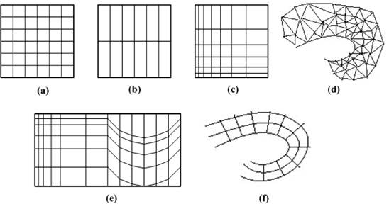
Figure 1.1: Grid types in volumetric data. a. Cartesian grid, b. Regular grid, c. Rectilinear grid, d. Curvilinear grid, e. Block structured grid, and f. Unstructured grid
In a rectilinear grid the cells are axis-aligned, but grid spacing along the axes are arbitrary. When such a grid has been non-linearly transformed while preserving the grid topology, the grid becomes curvilinear. Usually, the rectilinear grid defining the logical organization is called computational space, and the curvilinear grid is called physical space. Otherwise the grid is called unstructured or irregular. An unstructured or irregular volume data is a collection of cells whose connectivity has to be specified explicitly. These cells can be of an arbitrary shape such as tetrahedra, hexahedra, or prisms [14].
The array S only defines the value of some measured property of the data at discrete locations in space. A function f(x, y, z) may be defined over the volume in order to describe the value at any continuous location. The function f(x, y, z) = S(x, y, z) if (x, y, z) is a grid location, otherwise f(x, y, z) approximates the sample value at a location (x, y, z) by applying some interpolation function to S. There are many possible interpolation functions. The simplest interpolation function is known as zero-order interpolation, which is actually just a nearest-neighbor function [15]. The value at any location in the volume is simply the value of the closest sample to that location. With this interpolation method there is a region of a constant value around each sample in S. Since the samples in S are regularly spaced, each region is of a uniform size and shape. The region of the constant value that surrounds each sample is known as a voxel with each voxel being a rectangular cuboid having six faces, twelve edges, and eight corners.
Higher-order interpolation functions can also be used to define f(x, y, z) between sample points. One common interpolation function is a piecewise function known as first-order interpolation, or trilinear interpolation. With this interpolation function, the value is assumed to vary linearly along directions parallel to one of the major axes [14].
1.4. Voxels and cells
Volumes of data are usually treated as either an array of voxels or an array of cells. These two approaches stem from the need to resample the volume between grid points during the rendering process. Resampling, requiring interpolation, occurs in almost every volume visualization algorithm. Since the underlying function is not usually known, and it is not known whether the function was sampled above the Nyquist frequency, it is impossible to check the reliability of the interpolation used to find data values between discrete grid points. It must be assumed that common interpolation techniques are valid for an image to be considered valid.
Figure 1.2:Voxels. Each grid point has a sample value. Data values do not vary within voxels
The voxel approach dictates that the area around a grid point has the same value as the grid point (Figure 1.2). A voxel is, therefore, an area of non-varying value surrounding a central grid point. The voxel approach has the advantage that no assumptions are made about the behavior of data between grid points, only known data values are used for generating an image.
Figure 1.3: Cells. Data values do vary within cells. It is assumed that values between grid points can be estimated. Interpolation is used
The cell approach views a volume as a collection of hexahedra whose corners are grid points and whose value varies between the grid points (Figure 1.3). This technique attempts to estimate values inside the cell by interpolating between the values at the corners of the cell. Trilinear and tricubic are the most commonly used interpolation functions. Images generated using the cell approach, appear smoother than those images created with the voxel approach. However, the validity of the cell-based images cannot be verified [16].
1.5. Classification of Volume Rendering Algorithms
The object of this chapter is to give the general background of volume graphics together with a general classification. It is important to mention that there is not a complete agreement on a standard volume visualization vocabulary yet, a nomenclature is approaching consensus, where multiple terms exist for the same concept. And even a standard classification of volume visualization algorithms is not available. The classification of the algorithms given below is therefore not binding. All of the names of the algorithms are carefully taken into consideration and emphasized.
Volume visualization has been the most active sub-area of researches during last 20 years in scientific visualization. To be useful, volume visualization techniques must offer understandable data representations, quick data manipulation, and reasonably fast rendering. Scientific users should be able to change parameters and see the resultant image instantly. Few present day systems are capable of this type of performance; therefore researchers are still studying many new ways to use volume visualization effectively.
The rendering approaches differ in several aspects which can be used for their detailed classification in various ways [8, 9, 17-21]. Coarsely, volume visualization is done using two different approaches based on the portion of the volume raster set which they render; (Figure 1.4, Figure 1.5)
1.Surface rendering (or indirect volume rendering),
2.Volume rendering (or direct volume rendering).
Figure 1.4: Classification of volume visualization algorithms
Surface rendering (indirect rendering or surface oriented) algorithms are standard for nearly all 3D visualization problems. Surface oriented algorithms first fit geometric primitives to values in the data, and then render these primitives. The data values are usually chosen from an iso-surface, which is the set of locations in the data where the scalar field equals some value. In typical datasets from medical or scientific applications, the iso-surface forms a connected surface, such as the air/skin or brain/bone boundary in a CT dataset. With dedicated vector hardware, these models can be calculated very efficiently. Examples of surface oriented hardware are Reality Engine, HP, SUN, IBM, and PIXAR. Typical visualization problems to be solved in the medical context are e.g. tissues that have no defined surface or blood vessels whose size is close to the limit of imaging resolution. However surface oriented methods leave these problems unsolved.
An indirect volume rendering system transforms the data into a different domain (e.g., compression, boundary representation, etc.). Typically, the data is transformed into a set of polygons representing a level surface (or iso-surface); then conventional polygon rendering methods are used to project the polygons into an image [9]. Many methods exist for indirect volume rendering (surface rendering), which are defined as visualizing a volumetric dataset by first transferring the data into a different domain and rendering directly from the new domain. Indirect volume rendering can be classified as surface tracking, iso-surfacing, and domain-based rendering. Indirect methods are often chosen because of a particular form of hardware acceleration or because of a speed advantage [4, 10, 14, 17, 19-22].
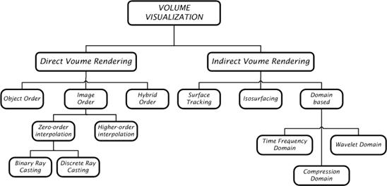
Figure 1.5:Detailed classification of volume rendering algorithms
Volume rendering (oriented) algorithmsrender every voxel in the volume raster directly, without conversion to geometric primitives or first converting to a different domain and then rendering from that domain. They usually include an illumination model which supports semi-transparent voxels; this allows rendering where every voxel in the volume is (potentially) visible. Each voxel contributes to the final 2D projection [18-21].
1.5.1. Surface tracking
Surface tracking is a surface reconstruction process that constructs a geometric surface from a volumetric dataset by following the faces of the voxels residing on the surface boundary. The boundary is defined by a thresholding, classification, or surface detection process. Given a threshold value, a closed contour is traced for each data slice (Figure 1.6) and then the contours in adjacent slices are connected and a tessellation, usually of triangles, is performed (Figure 1.7).
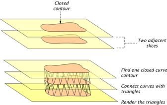
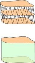
Figure 1.6:Contour tracing
Thresholdingis a segmentation operation that assigns a value 1 to a cell in Scene B if the corresponding cell in Scene A has an intensity that falls within a specified intensity interval and that assigns a value 0 to the cell otherwise. A less general thresholding operation is one in which a single intensity value is specified. If a cell's intensity in Scene A is above this value, it is assigned a value 1 in Scene B, and a value 0, otherwise. Classification is a process of converting a given set of scenes into a scene, all with identical domains, or into a non-binary shell. If the output is a scene, its cell intensity represents fuzziness or a membership value of the cell in the object of interest. In the case of a non-binary shell, the fuzziness or the membership value is retained as one of the property values associated with the shell elements.
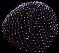
Figure 1.7:Examples of a contoured data that are tessellated
Surface tracking methods are well-known and effectively used for smooth surfaces. These algorithms are known as surface extraction, feature extraction, surface tiling, polygonization, tessellation, triangulation, tracing or meshing [23-31].
1.5.2. Iso-surfacing
Surface Detection (iso-surface) is an operation that given a scene outputs a connected surface as a binary shell. Connectedness means that within the output shell it is possible to reach to any shell element from any shell element without leaving the shell. If the input is a binary scene, the shell constitutes a connected interface between 1-cells and 0-cells. If the input is a (grey) scene, the interface between the interior and exterior of the structure is usually difficult to determine. Thresholding can be used to determine this interface, in which the shell constitutes essentially a connected interface between cells that satisfy the threshold criterion and cells that do not. In a particular thresholding operation specified by a single intensity value, the resulting surface is called an iso-surface. The common iso-surfacing algorithms are Opaque Cubes (Cuberille), Marching Cubes, Marching Tetrahedra, and Dividing Cubes.
1.5.2.1. Cuberille (Opaque cubes)
This algorithm was one of the first widely used methods for visualizing volume data. It was first proposed in [32], and involves deciding whether a particular volume element is a part of the surface or not. It simply visualizes the cells that are a part of the iso-surface. The first step in the cuberilles algorithm is to ensure that the volume is made up of cubic voxels. A large number of volume datasets consist of a stack of 2 dimensional slices [33]. If the distance between the slices is larger than the size of the pixels in the slice then the data must be resampled so that the gap between the slices is in the same size as the pixels. The second stage of the algorithm involves using a binary segmentation to decide which voxels belong to the object and which do not. This should, hopefully, produce a continuous surface of voxels through which the surface in the data passes. These voxels are joined together and the surface of the object is then approximated by the surfaces of the individual voxels which make up the surface.
The algorithm visualizes the cells that are intersected by the iso-surface in the following way. In the first stage, for each cell in the dataset intersected by the iso-surface, 6 polygons are generated representing the faces of the cell. In the second stage, for each polygon, polygon is rendered in an appropriate color.
The algorithm is easy and straightforward to implement. Finding and rendering the surface is fast. The first stage of the algorithm is parallelizable at the cell level. On the other hand, the final image might look jaggy, due to too less cells in the dataset, and the algorithm is fundamentally bad at showing small features. The blocky look of the final image can be reduced by using gradient shading during rendering.
1.5.2.2. Marching cubes
A variation on the Opaque Cubes (Cuberille) algorithm is provided by marching cubes [34]. The basic notion is that we can define a voxel by the pixel values at the eight corners of the cube. If one or more pixels of a cube have values less than a user-specified isovalue (threshold), and one or more have values greater than this value, we conclude that the voxel must contribute some component of the iso-surface. By determining which edges of the cube are intersected by the iso-surface, we can create triangular patches which divide the cube between regions within the iso-surface and regions outside. By connecting the patches from all cubes on the iso-surface boundary, we get a surface representation.
The basic idea of the algorithm is for each cell through which an iso-surface passes to create small polygons approximating the surface within the cell. For the threshold value, some voxels will be entirely inside or outside the corresponding iso-surface and some voxels will be intersected by the iso-surface. In the first pass of the algorithm the voxels that are intersected by the threshold value are identified. In the second pass these voxels are examined and a set of one or more polygons is produced, which are then output for rendering. Each of the 8 vertices of a voxel can be either inside or outside the iso-surface value. The exact edge intersection points are determined and using 15 predefined polygon sets the polygons are created (Figure 1.8).
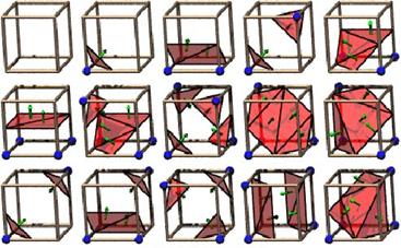
Figure 1.8: The 15 possible cases
The original algorithm proposed has several ambiguous cases which can lead to holes in the final image. These ambiguities occur either when a wrong decision is made about whether a vertex is inside or outside a surface, or if the triangles chosen do not fit together properly. A number of extensions have been proposed to the marching cubes algorithm to avoid the ambiguous cases. These include marching tetrahedra and dividing cubes. Both the marching cubes and opaque cubes (cuberille) algorithms involve an intermediate approximation of the surfaces in the data set using geometric primitives. This technique has a number of disadvantages:
1. There is a loss of accuracy when visualizing small or fuzzy details.
2. The assumptions which are made about the data may not necessarily be valid. This particularly applies to the assumption that the surfaces exist within the data to map the geometric primitives onto.
3. Unless the original information is stored along with the geometric representation, the information on the interior of the surfaces is lost.
The first two disadvantages listed here are directly linked to the requirement to map geometric primitives onto the data. While this method works well for some data sets, it breaks down when there are small details on a similar scale to the grid size in the data, and when well defined surfaces do not exist. These issues, along with the worry of losing the original data, led to the development of another class of algorithm, volume rendering.
One obvious problem with marching cubes is the amount of memory needed to store the resulting surface. Another problem arises when a filled space of voxels is not available. Depending on how the volume data was acquired there may be voids which need to be assigned values or circumnavigated in the surface generation algorithm. Any interpolated value used may reduce the validity of the resulting surface [33, 35, 36].
1.5.2.3. Dividing cubes
The Dividing cubes algorithm is an extension to or optimization of the Marching Cubes. It was designed to overcome the problem of the superfluous number of triangles with that algorithm[37]. Instead of, as in the marching cube algorithm, calculating the approximate iso-surface through a cell, the Dividing cubes algorithm first projects all cells that are intersected by the iso-surface to the image/screen space. If a cell projects to a larger area than a pixel it is divided into sub-cells and rendered as a surface point. Otherwise the whole cell is rendered as a surface point. After the surface points are determined, the gradients can be calculated, using interpolation between the original cells. With the given gradient, the shading can be calculated and finally the image can be rendered. Surface points can be rendered into the image buffer directly, because there are no intermediate surface primitives used. This is done by using standard computer graphics hidden-surface removal algorithms. This algorithm works far more faster than the marching cubes even when there is no any rendering hardware available. The algorithm is also parallelizable.
1.5.2.4. Marching tetrahedra
To perform the marching cubes algorithm, one way is to split a cube into some number of tetrahedra, and perform a marching tetrahedra algorithm [38-41]. The general idea here is so simple that the number of cases to consider in marching tetrahedra is far less than the number of cases in marching cubes. Cells can be divided into 5, 6, or 24 tetrahedra.
The Marching Tetrahedra Algorithm is the same as the Marching Cubes Algorithm up to the point that, the cube is divided into 5 tetrahedron instead of 15 as depicted in Figure 1.9.
As we step across the cubic space, we must alternate the decomposition of the cubes into tetrahedra. For a given tetrahedron, each of it's vertices are classified as either lying inside or outside the tetrahedron. There are originally 16 possible configurations. If we remove the two cases where all four vertex are either inside or outside the iso-value, we are left with 14 configurations. Due to symmetry there are only three real cases.

Figure 1.9: The Tetrahedra orientation within a cube
Based on these cases, triangles are generated to approximate the iso-surface intersection with the tetrahedron. Like the Marching Cubes Algorithm, when all of the triangles generated by marching these tetrahedrons are rendered across the cubic region, an iso-surface approximation is obtained.
The 5 Tetrahedra case requires flipping adjacent cells; otherwise anomalous, unconnected surfaces are encountered. The Marching Tetrahedra Algorithm has great advantages over the Marching Cubes Algorithm because the three cases are easier to deal with than 15, and the code is more manageable. Another advantage of using the Marching Tetrahedra Algorithm to approximate an iso-surface is that a higher resolution is achieved. Basically the cubes of the Marching Cubes Algorithm are subdivided into smaller geometries (tetrahedrons). More triangles are generated per cube, and these triangles are able to approximate the iso-surface better.
The disadvantages of the Marching Tetrahedra Algorithm is basically that because it sub-divides the cubes into 5 more sub-regions, the number of triangles generated by the Marching Tetrahedra Algorithm is greater than the number of triangles generated by the Marching Cubes Algorithm. While the Marching Tetrahedra Algorithm generates better iso-surfaces, the time to render the iso-surfaces is higher than that of the Marching Cubes Algorithm.
Factors that affect the performance of the marching tetrahedra algorithm are 3D grid size, grid resolution, number of objects, threshold, radius of influence for an individual object, and strength of an individual object.
1.5.3. Frequency domain rendering
The frequency domain rendering [42] applies the Fourier slice projection theorem [43, 44], which states that a projection of a 3D data volume from a certain view direction can be obtained by extracting a 2D slice perpendicular to that view direction out of the 3D Fourier spectrum and then inverse Fourier transforming it (Figure 1.10) [45].
It is well-known that the integral of a 1D signal is equal to the value of its spectrum at the origin. The Fourier projection slice theorem extends this notion to higher dimensions. For a 3D volume, the theorem states that the following two are a Fourier transform pair:
1. The 2D image obtained by taking line integrals of the volume along rays perpendicular to the image plane,
2. The 2D spectrum obtained by extracting a slice from the Fourier transform of the volume along a plane that includes the origin and is parallel to the image plane.
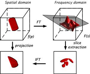
Figure 1.10: Frequency domain rendering
Using this theorem, once a volume data is Fourier transformed an (orthographic) image for any viewing direction can be obtained by extracting a 2D slice of the 3D spectrum at the appropriate orientation and than inverse Fourier transforming it. This approach obtains the 3D volume projection directly from the 3D spectrum of the data, and therefore reduces the computational complexity for volume rendering. The complexity is dominated by the 2D inverse Fourier transform that is O(N2logN). Since logN grows slowly, the advantage of this approach over spatial domain algorithms is greater at large data sizes [42].
Despite their theoretical speed advantage, frequency domain volume rendering algorithms suffer from several well-known problems such as a high interpolation cost, high memory usage, and the lack of depth information. The first two problems are technical in nature and several solutions are proposed. The lack of occlusion is fundamental and so far no projection-slice-theorem is known that reproduces the integro-differential equation approximated by volume rendering algorithms [42, 43, 45-47].
1.5.4. Compression domain rendering
As volume data sets grow bigger and larger, data compression algorithms are required to reduce the disk storage size, and potentially the memory size during rendering as well [48]. Data compression is an essential technology to achieve efficient volume visualization. Not only can it reduce the disk storage space with some effort, sometimes it can also be used to reduce the run-time memory requirement during the rendering process. There are basically two types of compression: lossless, and lossy compression. While lossless compression targets mainly at text documents, it can also be used to compress regular grids if data fidelity is crucial. Lossy compression, however, provides much higher compression efficiency, of course if data fidelity is not so crucial>
There are several possibilities to integrate volume data compression and volume rendering. The most naive way is to decompress the entire volume data set before rendering. This is simple and most flexible: different compression methods can be easily paired with different visualization methods. However there are three problems with this scheme [48]. The extra decompression time introduces a long start-up latency for the renderer. The data loading time, from the renderer’s point of view does not decrease despite the fact that the data sets are stored on disk in compressed form. The memory usage required for the renderer does not decrease, either. One might modify the renderer’s interface to eliminate the second problem by storing the uncompressed data set in memory without incurring additional disk I/O, but the first and third problems still remain.
To address the first issue, one can perform “on-the-fly” rendering during compression. This means the renderer can start working almost immediately as soon as the first “indivisible” unit of the data set is decompressed. This essentially reduces the start-up delay to the data loading time of the minimal data unit that the renderer can work on. In fact, the second issue is also solved, because the renderer does not need to hold the entire uncompressed data set but only the compressed form of it, by decompressing it on-the-fly. Furthermore, sometimes with the help of a “garbage collection” scheme, the memory requirement for rendering could also be reduced, thus solving the third problem as well. However, this scheme may require significant modification to the rendering algorithm and some coordination effort between the decompressor and the renderer.
Another scheme to address the start-up latency and memory requirement problems is to perform on-the-fly decompression during rendering. This usually means the data set was initially partitioned into units of the same or different sizes and during rendering only these units that the renderer need will be decompressed. As the final goal here is to produce a rendered image, the on-the-fly decompression scheme is favorable since unnecessary decompression work may be avoided. Although the on-the-fly decompression scheme requires only a minor modification effort to the renderer, it suffers from the following problem: In order for each data unit to be compressed/decompressed independently of each other, some kind of partitioning must be done. If all these partitions are mutually disjointed, then rendered images may exhibit a “blocky” effect. On the other hand, overlapping these partitions to remove these blocky artifacts leads to substantial severe storage overhead.
Another elegant way to integrate volume data compression and rendering is to perform rendering directly in the compression/transformed domain, thus avoiding decompression completely. Several methods have been proposed but each of them has its drawbacks: loss of quality, undesired artifacts, large storage overhead or exceedingly high implementation complexity.
Many compression algorithms applied to volume data sets are borrowed from the image compression world [49-53], simply because most of the time it can be directly generalized to deal with regular volume data. Among them are Discrete Fourier Transform, Discrete Cosine Transform, Vector Quantization, Fractal Compression, Laplacian Decomposition/Compression, and Wavelet Decomposition /Compression.
1.5.5. Wavelet domain rendering
A wavelet is a fast decaying function with zero averaging. The nice features of wavelets are that they have a local property in both spatial and frequency domain, and can be used to fully represent the volumes with a small number of wavelet coefficients [54]. Muraki [55] first applied wavelet transform to volumetric data sets, Gross et al. [56] found an approximate solution for the volume rendering equation using orthonormal wavelet functions, and Westermann [57] combined volume rendering with wavelet-based compression. However, all of these algorithms have not focused on the acceleration of volume rendering using wavelets. The greater potential of wavelet domain, based on the elegant multi-resolution hierarchy provided by the wavelet transform, is still far from being fully utilized for volume rendering. A possible research and development is to exploit the local frequency variance provided by wavelet transform and accelerate the volume rendering in homogeneous area.
1.5.6. Object order rendering
Direct volume rendering algorithms can be classified according to the order that the algorithm traverses the volume data [4, 10, 14, 20-22]. Object-order rendering is also called forward rendering, or object-space rendering or voxel space projection. The simplest way to implement viewing is to traverse all the volume regarding each voxel as a 3D point that is transformed by the viewing matrix and then projected onto a Z-buffer and drawn onto the screen. The data samples are considered with a uniform spacing in all three directions. If an image is produced by projecting all occupied voxels to the image plane in an arbitrary order, a correct image is not guaranteed. If two voxels project to the same pixel on the image plane, the one that was projected later will prevail, even if it is farther from the image plane than the earlier projected voxel. This problem can be solved by traversing the data samples in a back-to-front or front-to-back order. This visibility ordering is used for the detailed classification of object order rendering.
1.5.6.1. Back-to front (BTF) algorithm
Earliest rendering algorithms sorted the geometric primitives according to their distance to the viewing plane [58]. These algorithms solve the hidden surface problem by visiting the primitives in depth order, from farthest to nearest, and scan-converting each primitive into the screen buffer. Because of the order in which the primitives are visited, closer objects overwrite farther objects, which solve the hidden surface problem (at least as long as the primitives do not form a visibility cycle). Such methods are referred to as painter’s algorithms and as list-priority algorithms. By definition, any painter’s algorithm requires sorting the primitives. However, because of their structure, volume grids often afford a trivial sort, which simply involves indexing the volume elements in the proper order[19].
This algorithm is essentially the same as the Z-buffer method with one exception that is based on the observation that the voxel array is presorted in a fashion that allows scanning of its components in an order of decreasing distance from the observer. This avoids the need for a Z-buffer for hidden voxel removal considerations by applying the painter’s algorithm by simply drawing the current voxel on top of previously drawn voxels or by compositing the current voxel with the screen value [4, 10, 14, 22, 33, 59].
It is based on the simple observation that, given a volume grid and a view plane, for each grid axis there is a traversal direction that visits the voxels in the order of decreasing distances to the view plane. A 2D example of this is given in Figure 1.11 [19].
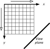
Figure 1.11: A 2D example of the BTF visibility ordering
Here the origin is the farthest point from the view plane, and traversing the grid in the order of increasing values of x and y always visits voxels in the order of decreasing distances. This extends naturally to 3D. The choice of which index changes fastest can be arbitrary – although.
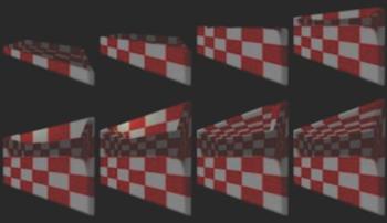
Figure 1.12: A cube rendered with the BTF visibility ordering. Note the visibility error along the top of the cube
BTF method can support efficient methods of accessing the volume data by taking into account how the data is stored on disk. It also allows rendering when only some slices but not the entire volume will fit into memory. While the BTF ordering correctly renders orthographic projections, it does not to work for perspective projections. This is demonstrated in Figure 1.12.
Westover gives the Westover back-to-front (WBTF) visibility ordering [60, 61]. The WBTF ordering is similar to the BTF ordering in that each grid axis is traversed in the direction that visits voxels in the order of decreasing distances to the view plane. The algorithm goes farther than the BTF technique in that it also chooses a permutation of the grid axes, such that the slowest changing axis is the axis that is most perpendicular to the view plane, while the quickest changing axis is the one that is most parallel to the view plane [19].
The V-BUFFER traversal ordering is similar to the WBTF traversal in that it processes the volume data in slices which are as parallel as possible to the view plane hence the orderings are the same. It differs in that it uses a more complicated “concentric sweep” to order the voxels in each slice. The sweep strictly orders the voxels according to increasing distances from the view plane. An example of the ordering for one slice is shown in Figure 1.13. When the viewing plane is beyond one corner of the slice, the voxels are visited in the diagonal pattern shown. This differs from the WBTF ordering, which accesses each slice in a scanline fashion, and hence does not visit the voxels in a strict distance ordering.
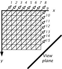
Figure 1.13: The V-BUFFER visibility ordering within each slice
1.5.6.2. Front-to back (FTB) algorithm
This algorithm is essentially the same as BTF only that now the voxels are traversed in an increasing distance order. It should be observed that while in the basic Z-buffer method it is impossible to support the rendition of semitransparent materials since the voxels are mapped to the screen in an arbitrary order. Compositing is based on a computation that simulates the passage of light through several materials. In this computation the order of materials is crucial. Therefore, translucency can easily be realized in both BTF and FTB in which objects are mapped to the screen in the order in which the light traverses the scene [4, 10, 14, 22, 33].
1.5.6.3. Splatting
The most important algorithm of the object order family is the splatting algorithm [61-63]. One way of achieving volume rendering is to try to reconstruct the image from the object space to the image space, by computing the contribution of every element in the dataset to the image. Each voxel's contribution to the image is computed and added to the other contributions. The algorithm works by virtually “throwing” the voxels onto the image plane. In this process every voxel in the object space leaves a footprint in the image space that will represent the object. The computation is processed by virtually slice by slice, and by accumulating the result in the image plane.
The first step is to determine in what order to traverse the volume. The closest face (and corner) to the image plane is determined. Then the closest voxels are splatted first. Each voxel is given a color and opacity according to the look up tables set by the user. These values are modified according to the gradient.
Next, the voxel is projected into the image space. To compute the contribution for a particular voxel, a reconstruction kernel is used. For an orthographic projection a common kernel is a round Gaussian (Figure 1.14). The projection of this kernel into the image space (called its footprint) is computed. The size is adjusted according to the relative sizes of the volume and the image plane so that the volume can fill the image. Then the center of the kernel is placed at the center of the voxel's projection in the image plane (note that this does not necessarily correspond to a pixel center). Then the resultant shade and opacity of a pixel is determined by the sum of all the voxel contributions for that pixel, weighted by the kernel.
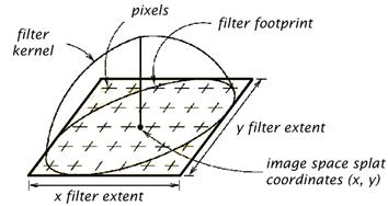
Figure 1.14: The splatting process reconstruction and resampling with the 2D filter kernel
1.5.7. Image order rendering
Image-order rendering (also called backward mapping, ray casting, pixel space projection, or image-space rendering) techniques are fundamentally different from object-order rendering techniques. Instead of determining how a data sample affects the pixels on the image plane, we determine the data samples for each pixel on the image plane, which contribute to it.
In ray casting, rays are cast into the dataset. Each ray originates from the viewing (eye) point, and penetrates a pixel in the image plane (screen), and passes through the dataset. At evenly spaced intervals along the ray, sample values are computed using interpolation. The sample values are mapped to display properties such as opacity and color. A local gradient is combined with a local illumination model at each sample point to provide a realistic shading of the object. Final pixel values are found by compositing the color and opacity values along the ray. The composition models the physical reflection and absorption of light [4].
In ray casting, because of high computational requirements of volume rendering, the data needs to be processed in a pipelined and parallel manner. They offer a flexibility for algorithmic optimizations, but accessing the volume memory in a non-predictable manner significantly slows down the memory performance. The data flow diagram of a ray casting system is shown in Figure 1.15.
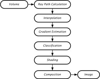
Figure 1.15:The data flow diagram of a ray casting system
Any ray casting implementation requires a memory system, ray path calculation, interpolation, gradient estimation, classification, shading, and composition [4, 64]. The memory system provides the necessary voxel values at a rate which ultimately dictates the performance of the architecture. The ray-path calculation determines the voxels that are penetrated by a given ray: it is tightly coupled with the organization of the memory system. The interpolation estimates the value at a re-sample location using a small neighborhood of voxel values. The gradient estimation estimates a surface normal using a neighborhood of voxels surrounding the re-sample location. The classification maps interpolated sample values and the estimated surface normal to a color and opacity. The shading uses the gradient and classification information to compute a color that takes the interaction of light into account on the estimated surfaces in the dataset. The composition uses shaded color values and the opacity to compute a final pixel color to display. Ray casting can be classified into two sub-classes according to the level of interpolation used [14]:
1. Algorithms that use a zero order interpolation,
2. Algorithms that use a higher order interpolation.
Algorithms that use a zero order interpolation are Binary Ray Casting, and Discrete Ray Casting. Binary Ray Casting was developed to generate images of surfaces contained within binary volumetric data without the need to explicitly perform boundary detection and hidden-surface removal. For each pixel on the image plane, a ray is cast from that pixel to determine if it intersects the surface contained within the data. In order to determine the first intersection along the ray a stepping technique is used where the value is determined at regular intervals along the ray until the object is intersected. Data samples with a value of 0 are considered to be the background while those with a value of 1 are considered to be a part of the object [65]. In Discrete Ray Casting, instead of traversing a continuous ray and determining the closest data sample for each step, a discrete representation of the ray is traversed [14]. This discrete ray is generated using a 3D Bresenham-like algorithm or a 3D line scan-conversion (voxelization) algorithm [66, 67]. As in the previous algorithms, for each pixel in the image plane, the data samples which contribute to it need to be determined. This could be done by casting a ray from each pixel in the direction of the viewing ray. This ray would be discretized (voxelized), and the contribution from each voxel along the path is considered when producing the final pixel value [68].
Algorithms that use a higher order interpolation are the image order volume rendering algorithm of Levoy, V-Buffer image order ray casting , and V-Buffer cell-by-cell processing. The image-order volume rendering algorithm developed by Levoy [69] states that given an array of data samples , two new arrays which define the color and opacity at each grid location can be generated using preprocessing techniques. The interpolation functions which specify the sample value, color, and opacity at any location in volume, are then defined by using transfer functions proposed by him. Generating the array of color values involves performing a shading operation. In V-Buffer image order ray casting method, rays are cast from each pixel on the image plane into the volume. For each cell in the volume along the path of this ray, a scalar value is determined at the point where the ray first intersects the cell. The ray is then stepped along until it traverses the entire cell, with calculations for scalar values, shading, opacity, texture mapping, and depth cuing performed at each stepping point. This process is repeated for each cell along the ray, accumulating color and opacity, until the ray exits the volume, or the accumulated opacity reaches to unity. At this point, the accumulated color and opacity for that pixel are stored, and the next ray is cast. The goal of this method is not to produce a realistic image, but instead to provide a representation of the volumetric data which can be interpreted by a scientist or an engineer. In V-Buffer cell-by-cell processing method each cell in the volume is processed in a front-to-back order [14, 70]. Processing begins on the plane closest to the viewpoint, and progresses in a plane-by-plane manner. Within each plane, processing begins with the cell closest to the viewpoint, and then continues in the order of increasing distance from the viewpoint. Each cell is processed by first determining for each scan line in the image plane which pixels are affected by the cell. Then, for each pixel an integration volume is determined. This process continues in a front-to-back order, until all cells have been processed, with an intensity accumulated into pixel values.
1.5.8. Hybrid order rendering
This approach to volume rendering adopts the advantages of both object-order and image-order algorithms, and is known as hybrid projection. They may be a combination of both image order approach and object order approach or do not fall into either one of them [48]. V-Buffer algorithm [70] is given as an example of hybrid traversal in [20, 48, 71]. V-Buffer algorithm divides data set into cells, and render it cell-by-cell, which makes it an object order method. But within each cell ray-casting is used, therefore it is a hybrid approach. In [22] the volume data set is rendered by first shearing the volume slice to make ray traversal trivial, and then warps the intermediate image to the final image. EM-Cube [72] is a parallel ray casting engine that implements a hybrid order algorithm [71]. The most popular hybrid algorithm is the shear-warp factorization.
1.5.8.1. The shear-warp factorization
Image-order algorithms have the disadvantage that the spatial data structure must be traversed once for every ray, resulting in redundant computations [69]. Object-order algorithms operate through the volume data in the storage order making it difficult to implement an early ray termination, an effective optimization in ray-casting algorithms [73]. The shear-warp algorithm [22] combines the advantages of image-order and object-order algorithms. The method is based on a factorization of the viewing matrix into a 3D shear parallel to the slices of the volume data, a projection to form a distorted intermediate image, and a 2D warp to produce the final image. The advantage of shear-warp factorizations is that scanlines of the volume data and scanlines of the intermediate image are always aligned.
The arbitrary nature of the transformation from object space to image space complicates efficient, high-quality filtering and projection in object-order volume rendering algorithms. This problem is solved by transforming the volume to an intermediate coordinate system for which there is a very simple mapping from the object coordinate system and which allows an efficient projection. The intermediate coordinate system is called sheared object space and by construction, in sheared object space all viewing rays are parallel to the third coordinate axis.
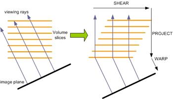
Figure 1.16: A volume is transformed to sheared object space for a parallel projection by translating each slice. The projection in sheared object space is simple and efficient
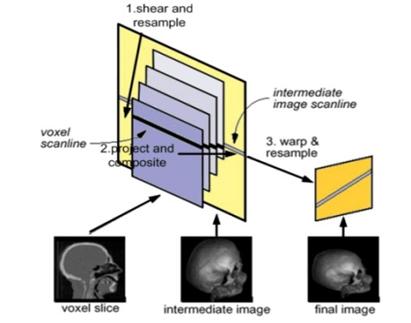
Figure 1.17: The shear-warp algorithm includes three conceptual steps: shear and resample the volume slices, project resampled voxel scanlines onto intermediate image scanlines, and warp the intermediate image into the final image
Figure 1.16 and Figure 1.17 illustrates the transformation from object space to sheared object space for a parallel projection. The volume is assumed to be sampled on a rectilinear grid. After the transformation the volume data is sheared parallel to the set of slices that is most perpendicular to the viewing direction and the viewing rays are perpendicular to the slices.
There are three variations of shear warp algorithm. Parallel projection rendering algorithm is optimized for parallel projections and assumes that the opacity transfer function does not change between renderings, but the viewing and shading parameters can be modified. Perspective projection rendering algorithm supports perspective projections. Fast classification algorithm allows the opacity transfer function to be modified as well as the viewing and shading parameters, with a moderate performance penalty.
1.6. Optimization in Volume Rendering
Volume rendering can produce informative images that can be useful in data analysis, but a major drawback of the techniques is the time required to generate a high-quality image. Several volume rendering optimizations are developed which decrease rendering times, and therefore increase interactivity and productivity It is obvious that one can not hope to have a real time volume rending in the near future without investing time, effort, and ingenuity in accelerating the process through software optimizations and hardware implementations. There are five main approaches to overcoming this seemingly insurmountable performance barrier [10]:
1. Data reduction by means of model extraction or data simplification,
2. software-based algorithm optimization and acceleration,
3. implementation on general purpose parallel architectures,
4. use of contemporary off-the-shelf graphics hardware, and
5. realization of special-purpose volume rendering engines.
1.6.1. Task and data decomposition
Since the work is essentially defined as “operations on data”, the choice of task decomposition has a direct impact on data access patterns. On distributed memory architectures, where remote memory references are usually much more expensive than local memory references, the issues of task decomposition and data distribution are inseparable. Shared memory systems offer more flexibility, since all processors have an equal access to the data. While data locality is still important in achieving good caching performance, the penalties for global memory references tend to be less severe, and static assignment of data to processors is not generally required.
There are two main strategies for task decomposition [74]. In an object-parallel approach, tasks are formed by partitioning either the geometric description of the scene or the associated object space. Rendering operations are then applied in parallel to subsets of the geometric data, producing pixel values which must then be integrated into a final image. In contrast, image-parallel algorithms reverse this mapping. Tasks are formed by partitioning the image space, and each task renders the geometric primitives which contribute to the pixels which it has been assigned. To achieve a better balance among the various overheads, some algorithms adopt a hybrid approach, incorporating features of both object- and image-parallel methods. These techniques partition both the object and image spaces, breaking the rendering pipeline in the middle and communicating intermediate results from object rendering tasks to image rendering tasks[75].
Volume rendering algorithms typically loops through the data, calculating the contribution of each volume sample to pixels on the image plane. This is a costly operation for moderate to large sized data, leading to rendering times that are non-interactive. Viewing the intermediate results in the image plane may be useful, but these partial image results are not always representatives of the final image. For the purpose of interaction, it is useful to be able to generate a lower quality image in a shorter amount of time, which is known as data simplification. For data sets with binary sample values, bits could be packed into bytes such that each byte represents a 2´2´2 portion of the data [65]. The data would be processed bit-by-bit to generate the full resolution image, but lower resolution image could be generated by processing the data byte-by-byte. If more than four bits of the byte are set, the byte is considered to represent an element of the object, otherwise it represents the background. This will produce an image with one-half the linear resolution in approximately one eighth the time [14].
1.6.2. Software-based algorithm optimization and acceleration
Software based algorithm optimizations are divided into two broad groups according to the rendering methods they use, that is optimization methods for object-space rendering and image-space rendering. The methods that have been suggested to reduce the amount of computations needed for the transformation by exploiting the spatial coherency between voxels for object-space rendering are [59]:
1. Recursive “divide and conquer”,
2. pre-calculated tables,
3. incremental transformation, and
4. shearing-based transforms.
The major algorithmic strategy for parallelizing volume rendering is the divide-and-conquer paradigm. The volume rendering problem can be subdivided either in data space or in image space. Data-space subdivision assigns the computation associated with particular sub volumes to processors, while image-space subdivision distributes the computation associated with particular portions of the image space. This method exploits coherency in voxel space by representing the 3D volume by an octree. A group of neighboring voxels having the same value may, under some restrictions, be grouped into a uniform cubic sub volume. This aggregate of voxels can be transformed and rendered as a uniform unit instead of processing each of its voxels.
The table-driven transformation method [59] is based on the observation that volume transformation involves the multiplication of the matrix elements with integer values which are always in the range of volume resolution. Therefore, in a short preprocessing stage each matrix element is allocated a table. All the multiplication calculations required for the transformation matrix multiplication are stored into a look-up table. The transformation of a voxel can then be accomplished simply by accessing the look-up table, the entry accessed in the table depending on the xyz coordinates of the voxel. During the transformation stage, coordinate by matrix multiplication is replaced by table lookup [10, 21].
The incremental transformation method is based on the observation that the transformation of a voxel can be incrementally computed given the transformed vector of the voxel. To employ this approach, all volume elements, including the empty ones, have to be transformed [76]. This approach is especially attractive for vector processors since the transformations of the set of voxels can be computed from the transformation of the vector by adding, to each element in this vector. Machiraju and Yagel [77] exploit coherency within the volume to implement a novel incremental transformation scheme. A seed voxel is first transformed using the normal matrix-vector multiplication. All other voxels are then transformed in an incremental manner with just three extra additions per coordinate.
The shearing algorithm decomposes the 3D affine transformation into five 1D shearing transformations. The major advantage of this approach is its ability (using simple averaging techniques) to overcome some of the sampling problems causing the production of low quality images. In addition, this approach replaces the 3D transformation by five 1D transformations which require only one floating-point addition each [10].
The image-space optimization methods are based on the observation that most of the existing methods for speeding up the process of ray casting rely on one or more of the following principles:
1. Pixel-space coherency,
2. object-space coherency,
3. inter-ray coherency,
4. frame coherency, and
5. space-leaping.
Pixel-space coherency means that there is a high coherency between pixels in the image space. It is highly probable that between two pixels having identical or similar color we will find another pixel having the same or similar color. Therefore, it might be the case that we could avoid sending a ray for such obviously identical pixels [10, 11, 20, 78].
Object-space coherency means that there is coherency between voxels in the object space. Therefore, it should be possible to avoid sampling in 3D regions having uniform or similar values. In this method the ray starts sampling the volume in a low frequency (i.e., large steps between sample points). If a large value difference is encountered between two adjacent samples, additional samples are taken between them to resolve ambiguities in these high frequency regions [10, 11, 20, 79]
Inter-ray coherency means that, in parallel viewing, all rays have the same form and there is no need to reactivate the discrete line algorithm for each ray. Instead, we can compute the form of the ray once and store it in a data structure called the ray-template. Since all the rays are parallel, one ray can be discretized and used as a ‘‘template’’ for all other rays [14, 20].
Frame coherency means that when an animation sequence is generated, in many cases, there is not much difference between successive images. Therefore, much of the work invested to produce one image may be used to expedite the generation of the next image [10, 11, 20, 80, 81].
The most prolific and effective branch of volume rendering acceleration techniques involve the utilization of the fifth principle: speeding up ray casting by providing efficient means to traverse the empty space, that is space leaping [80]. The passage of a ray through the volume is two phased. In the first phase the ray advances through the empty space searching for an object. In the second phase the ray integrates colors and opacities as it penetrates the object. Since the passage of empty space does not contribute to the final image it is observed that skipping the empty space could provide a significant speed up without affecting the image quality [10, 11, 20].
1.6.3. Parallel and distributed architectures
The need for interactive or real-time response in many applications places additional demands on processing power. The only practical way to obtain the needed computational power is to exploit multiple processing units to speed up the rendering task, a concept which has become known as parallel rendering.
Several different types of parallelism can be applied in the rendering process. These include functional parallelism, data parallelism, and temporal parallelism. Some are more appropriate to specific applications or specific rendering methods, while others have a broader applicability. The basic types can also be combined into hybrid systems which exploit multiple forms of parallelism [74, 75, 82-91].
One way to obtain parallelism is to split the rendering process into several distinct functions which can be applied in series to individual data items. If a processing unit is assigned to each function (or group of functions) and a data path is provided from one unit to the next, a rendering pipeline is formed. As a processing unit completes work on one data item, it forwards it to the next unit, and receives a new item from its upstream neighbor. Once the pipeline is filled, the degree of parallelism achieved is proportional to the number of functional units. The functional approach works especially well for polygon and surface rendering applications.
Instead of performing a sequence of rendering functions on a single data stream, it may be preferable to split the data into multiple streams and operate on several items simultaneously by replicating a number of identical rendering units. The parallelism achievable with this approach is not limited by the number of stages in the rendering pipeline, but rather by economic and technical constraints on the number of processing units which can be incorporated into a single system.
In animation applications, where hundreds or thousands of high-quality images must be produced for a subsequent playback, the time to render individual frames may not be as important as the overall time required to render all of them. In this case, parallelism may be obtained by decomposing the problem in the time domain. The fundamental unit of work is a complete image, and each processor is assigned a number of frames to render, along with the data needed to produce those frames [75].
It is certainly possible to incorporate multiple forms of parallelism in a single system. For example, the functional- and data-parallel approaches may be combined by replicating all or a part of the rendering pipeline.
1.6.4. Commercial graphics hardware
One of the most common resources for rendering is off-the-shelf graphics hardware. However, these polygon rendering engines seem inherently unsuitable to the task. Recently, some new methods have tapped to this rendering power by either utilizing texture mapping capabilities for rendering splats, or by exploiting solid texturing capabilities to implement a slicing-based volume rendering [92, 93]. The commercially available solid texturing hardware allows mapping of volumes on polygons using these methods. These 3D texture maps are mapped on polygons in 3D space using either zero order or first order interpolation. By rendering polygons, slicing the volume and perpendicular to the view direction one generates a view of a rectangular volume data set [22].
1.6.5. Special purpose hardware
To fulfill the special requirements of high-speed volume visualization, several architectures have been proposed and a few have been built. The earliest proposed volume visualization system was the “Physician’s Workstation” which proposed real-time medical volume viewing using a custom hardware accelerator. The Voxel Display Processor (VDP) was a set of parallel processing elements. A 643 prototype was constructed which generated 16 arbitrary projections each second by implementing depth-only-shading. Another system which presented a scalable method was SCOPE architecture. It was also implementing the depth-only-shading scheme.
The VOGUE architecture was developed at the University of Tübingen, Germany. A compact volume rendering accelerator, which implements the conventional volume rendering ray casting pipeline proposed in [69], originally called the Voxel Engine for Real-time Visualization and Examination (VERVE), achieved 2.5 frames/second for 2563 datasets.
The design of VERVE [94] was reconsidered in the context of a low cost PCI coprocessor board. This FPGA implementation called VIZARD was able to render 10 perspective, ray cast, grayscale 256 x 200 images of a 2562 x 222 volume per second.
VIZARD II architecture is at the University of Tübingen to bring interactive ray casting into the realm of desktop computers and was designed to interface to a standard PC system using the PCI bus. It sustained a frame rate of 10 frames/second in a 2563 volume (Figure 1.18) [4, 9].
Figure 1.18 : VIZARD II co-processor card
In DOGGETT system an array-based architecture for volume rendering is described. It performs ray casting by rotating planes of voxels with a warp array, then passing rays through it in the ray array. The estimated performance for an FPGA implementation is 15 frames/second yielding 3842 images of 2563 data sets [9].
The VIRIM architecture [17] has been developed and assembled in the University of Mannheim which implements the Heidelberg ray tracing model [95], to achieve real-time visualization on moderate sized (256 x 256 x 128) datasets with a high image quality. VIRIM was capable of producing shadows and supports perspective projections. One VIRIM module with four boards has been assembled and achieved 2.5 Hz frame rates for 256 x 256 x 128 datasets. To achieve interactive frame rates, multiple rendering modules have to be used; however, dataset duplication was required. Four modules (16 boards) were estimated to achieve 10 Hz for the same dataset size, and eight modules (32 boards) were estimated to achieve 10 Hz for 2563 datasets [4, 9].
VIRIM II [18] improved on VIRIM by reducing the memory bottleneck. The basic design of a single memory interface was unchanged. To achieve higher frame rates or to handle higher resolutions, multiple nodes must be connected on a ring network that scales with the number of nodes. It was predicted that using 512 nodes, a system could render 20483 datasets at 30 Hz. [4, 9].
The hierarchical, object order volume rendering architecture BELA, with eight projection processors and image assemblers, was capable of rendering a 2563 volume into an imageat a 12 Hz rendering rate [72].
The Distributed Volume Visualization Architecture [9], DIV2A, was an architecture that performed conventional ray casting with a linear array of custom processors. To achieve 20Hz frame rates with a 2563 volume, 16 processing elements using several chips each were required.
The volume rendering architecture with the longest history is the Cube family. Beginning with Cube-1 and spanning to Cube-4 and beyond, the architecture provides a complete, real-time volume rendering visualization system. A mass market version of Cube-4 was introduced in 1998 providing real-time volume rendering of 2563 volumes at 30 Hz for inclusion in a desktop personal computer [9].
The Cube-1 concept was proven with a wire-wrapped prototype (Figure 1.19). 2D projections were generated at a frame rate of 16 Hz for a 5123 volume. The main problems with the implementation of Cube-1 were the large physical size and the long settling time. To improve these characteristics, Cube-2 was developed [9].
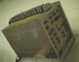
Figure 1.19: A 163 resolution prototype of Cube-1 architecture
Cube-2 [96] implemented a 163 VLSI version of Cube-1 (Figure 1.20). A single chip contained all the memory and processing of a whole Cube-1 board.
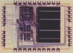
Figure 1.20:A 163 resolution Cube-2 VLSI implementation
Although the prior Cube designs were fast, the foundations of volume sampling and rendering were not fully developed so the architecture was unable to provide higher order sampling and shading. Cube-3 [97] improved the quality of rendering by supporting full 3D interpolation of samples along a ray, accurate gray-level gradient estimation, and flexible volumetric shading and provided real-time rendering of 5123 volumes.
Due to the capability of providing real-time rendering, the cost and size of the Cube-3 was unreasonable. This prompted the development of Cube-4 [98] which avoided all global communication, except at the pixel level and achieved rendering in 1283 datasets in 0.65 seconds at 0.96 MHz processing frequency. There is also a new version Cube-4L which is currently being implemented by Japan Radio Co. as part of a real-time 3D ultrasound scanner [9, 99].
EM-Cube is a commercial version of the high-performance Cube-4 volume rendering architecture that was originally developed at the State University of New York at Stony Brook, and is implemented as a PCI card for Windows NT computers. EM-Cube is a parallel projection engine with multiple rendering pipelines. Eight pipelines operating in parallel can process 8 x 66 x 106 or approximately 533 million samples per second. This is sufficient to render 2563 volumes at 30 frames per second[4, 9, 71]. It does not support perspective projections.
VolumePro [100], the first single chip rendering system is developed at SUNY Stony Brook and is based on the Cube-4 volume rendering architecture. VolumePro is the commercial implementation of EM-Cube, and it makes several important enhancements to its architecture and design. VolumePro is now available on a low cost PCI board delivering the best price/performance ratio of any available volume rendering system (Figure 1.21 [101].
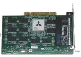
Figure 1.21: The VolumePro PCI card
1.7. Conclusion
In this chapter, we have reviewed the general background of volume rendering and found out what had been done in the literature. Volume rendering techniques allows us to fully reveal the internal structure of 3D data, including amorphous and semi-transparent features. It encompasses an array of techniques for displaying images directly from 3D data. Surface rendering algorithms fit geometric primitives to the data and then render, making this approach unattractive. Direct rendering methods render volumetric datasets directly without converting to any intermediate geometric representation, thus, it has become a key technology in the visualization of scientific volumetric data.
1.8. REFERENCES
[1] Foley, J.D., Dam, A.V., Feiner S.K., and Hughes J.F. (1990). Computer Graphics: Principles and Practice. (2th ed.). Massachusetts: Addison-Wesley Publishing Company.
[2] Hearn, D., and Baker, M.P. (1997). Computer Graphics C Version. (2th ed.). New Jersey: Prentice Hall.
[3] Foley, J.D., Dam, A.V., Feiner S.K., and Hughes J.F., Phillips R.L. (1995). Introduction to Computer Graphics. Massachusetts: Addison-Wesley.
[4] Ray, H., Pfister, H., Silver, D., and Cook, T.A. (1999). Ray Casting Architectures for Volume Visualization. IEEE Transactions on Visualization and Computer Graphics, 5(3), 210-233
[5] Jones, M.W. (1996). The Production of Volume Data fram Triangular Meshes Using Voxelization. Computer Graphics Forum, 15(5), 311-318
[6] Cooke, J.M., Zyda, M.J., Pratt, D.R., and McGhee, R.B. (1992). NPSNET: Flight Simulation Dynamic Modeling Using Quaternions. Teleoperations and Virtual Environments, 1(4), 404-420
[7] Schalkoff, R.J. (1989). Digital Image Processing and Computer Vision. Singapore: John Wiley & Sons Publishing.
[8] Jürgen, H., Manner, R., Knittel, G., and Strasser, W. (1995). Three Architectures for Volume Rendering. International Journal of the Eurographics Association, 14, 111-122
[9] Dachille, F. (1997). Volume Visualization Algorithms and Architectures. Research Proficiency Exam, SUNY at Stony Brook
[10] Yagel, R. (1996). Towards Real Time Volume Rendering. Proceedings of GRAPHICON' 96, 230-241
[11] Yagel, R. (1998). Data Visualization Techniques. C. Bajaj (Ed.), John Wiley & Sons. Efficient Techniques for Volume Rendering of Scalar Fields.
[12] Ma, K.L., and Crockett, T.W. (1997). A Scalable Parallel Cell-Projection Volume Rendering Algorithm for Three-Dimensional Unstructured Data. IEEE Parallel Rendering Symposium, 95-104
[13] Kaufman, A.E. (1997). Volume Visualization: Principles and Advances. SIGGRAPH '97, 23-35
[14] Kaufman, A.E. (1994). Voxels as a Computational Representation of Geometry. in The Computational Representation of Geometry SIGGRAPH '94 Course Notes
[15] Press, W.H., Teulkolsky, S.A., Vetterling, W.T., Flannery, B.P. (1997). Numerical Recipes in C. (2th ed.). Cambridge: Cambridge University Press.
[16] Elvins, T.T. (1992). A Survey of Algorithms for Volume Visualization. Computer Graphics, 26 (3), 194-201
[17] Günther, T., Poliwoda, C., Reinhart, C., Hesser, J., and Manner, J. (1994). VIRIM: A Massively Parallel Processor for Real-Time Volume Visualization in Medicine. Proceedings of the 9th Eurographics Hardware Workshop, 103-108
[18] Boer, M.De, Gröpl, A., Hesser, J., and Manner, R. (1996). Latency-and Hazard-free Volume Memory Architecture for Direct Volume Rendering. Eurographics Workshop on Graphics Hardware, 109-119
[19] Swan, J.E. (1997). Object Order Rendering of Discrete Objects. PhD. Thesis, Department of Computer and Information Science, The Ohio State University
[20] Yagel, R. (1996). Classification and Survey of Algorithms for Volume Viewing. SIGGRAPH tutorial notes (course no. 34)
[21] Law,A. (1996). Exploiting Coherency in Parallel Algorithms for Volume Rendering. PhD. Thesis, Department of Computer and Information Science, The Ohio State University
[22] Lacroute, P., and Levoy, M. (1994). Fast Volume Rendering Using a Shear-Warp Factorization of the Viewing Transform. Computer Graphics Proceedings Annual Conference Series ACM SIGGRAPH, 451-458.
[23] Bloomenthal, J. (1997) Introduction to Implicit Surfaces. In J. Bloomenthal (Ed.), Surface Tiling.
[24] Balendran, B. (1999). A Direct Smoothıng Method For Surface Meshes. Proceedings of 8th International Meshing Roundtable, 189-193
[25] Bloomenthal, J. (1988). Polygonization of Implicit Surfaces. Computer Aided Geometric Design, 5(00), 341-355
[26] Jondrow, M. (2000). A Survey of Animation Related Implicit Surface Papers. Computer Graphics Course Notes, The University of George Washington
[27] Lin, K. (1997). Surface and 3D Triangular Meshes from Planar Cross Sections. PhD Thesis, Purdue University
[28] Azevedo, E.F.D. (1999). On Adaptive Mesh Generation in Two-Dimensions. Proceedings, 8th International Meshing Roundtable, 109-117
[29] Miller, J.V. (1990). Geometrically Deformed Models for the Extraction of Closed Shapes from Volume Data. PhMs. Thesis, Rensselaer Polytechnic Institute
[30] Gross, M.H., Gatti, R., and Staadt, O. (1995). Fast Multiresolution Surface Meshing. Proceedings of IEEE Visualization '95, 135-142
[31] Borouchaki, H., Hecht, F., Saltel, E., and George, P.L. (1995). Reasonably Efficient Delaunay-based Mesh Generator in 3 Dimensions. Proceedings of 4th International Meshing Roundtable, 3-14
[32] Herman, G.T., and Liu, H.K. (1979). Optimal Surface Reconstruction from Planar Contours. Computer Graphics and Image Processing, 1-121
[33] Roberts, J.C. (1993). An Overview of Rendering from Volume Data including Surface and Volume Rendering. Technical Report 13-93*, University of Kent, Computing Laboratory, Canterbury, UK
[34] Lorenson, W.E., and Cline, H.E. (1987). Marching Cubes: A High Resolution 3D Surface Construction Algorithm. Computer Graphics, 21(4), 163-169
[35] Montani, C., Scateni, R., and Scopigno, R. (1994). Discretized Marching Cubes. Visualization '94 Proceedings, 281-287
[36] Smemoe, C.M. (2000). Volume Visualization and Recent Research in the Marching Cubes Approach. Cource Notes of School of Engineering, Cardiff University, UK
[37] Cline, H.E., Lorensen, W.E., Ludke, S., Crawford, C.R., and Teeter, B.C.(1988). Two Algorithms for the Three-Dimensional Reconstruction of Tomograms. Medical Physics, 15(3), 320-327
[38] Cignoni, P., Montani, C., Puppo, E., and Scopigno, R. (1996). Optimal Isosurface Extraction from Irregular Volume Data. Proceedings of Volume Visualization Symposium, 31-38
[39] Cignoni, P., Montani, C., and Scopigno, R. (1998). Mathematical Visualization. In Hege, H.C. and Polthier, K. (Eds.), Tetrahedra Based Volume Visualization, 3-18
[40] Treece, G.M., Prager, R.W., and Gee, A.H. (1998). Regularised Marching Tetrahedra: Improved Iso-Surface Extraction., Computers and Graphics, 104-110.
[41] Staadt, G. O., and Gross, M.H. (1998). Progressive Tetrahedralizations. Proceedings of IEEE Visualization '98,397-402
[42] Totsuka, T., and Levoy, M. (1993). Frequency Domain Volume Rendering. Computer Graphics Proceedings, Annual Conference Series, 271-278.
[43] Oppenheim, A.V., and Schafer, R.W. (1975) Digital Signal Processing. London: Prentice Hall International Inc.
[44] Lim, J.S. (1990). Two Dimensional Signal and Image Processing. London: Prentice Hall International Inc.
[45] Levoy, M. (1992). Volume Rendering Using Fourier Slice Theorem. IEEE Computer Graphics and Applications, 3, 202-212
[46] Dunne, S., Napel, S., and Rutt, B. (1990). Fast Reprojection of Volume Data. Proc. First Conference on Visualization in Biomedical Computing, IEEE Computer Society Press, 11-18
[47] Malzbender, T. (1993). Fourier Volume Rendering. ACM Transactions on Graphics, 12(3), 233-250
[48] Yang, C. (2000). Integration of Volume Visualization and Compression: A Survey. The Visual Computer, 11(6), 225-242
[49] Baharov, Z., Krupnik, H., Malah, D., and Karnin, E. (1996). Fractal Image Encoding and Analysis. In Y. Fisher (Ed.), A Multi-resolution Framework for Fractal Image Representation and its Applications.
[50] Fisher, Y. (1992). Fractal Image Compression : SIGGRAPH’92 Course Notes
[51] Fisher, Y., Rogovin, D., and Shen, T.P. (1994). A Comparison of Fractal Methods with DCT and Wavelets. Neural and Stochastic Methods in Image and Signal Processing III volume Proc. SPIE ,23, 04-16
[52] Gray, R.M. (1984, April). Vector Quantization. IEEE ASSP Magazine, 14-29
[53] Chiueh, T., Yang, C., and He, T. (1997). Integrated Volume Compression and Visualization. Proceedings of Visualization '97, 329-336
[54] Gross, M.H., Lippert, L., Dittrich, R., and Haring, S. (1997). Two Methods for Wavelet-Based Volume Rendering. Computers and Graphics, 21(2), 237-252
[55] Muraki, S. (1993). Volume Data and Wavelet Transform. IEEE Computer Graphics & Applications, 13(4), 50-56
[56] Gross, M., Lippert, L., Dreger, A., and Koch., R. (1995). A New Method to Approximate the Volume Rendering Equation Using Wavelets and Piecewise Polynomials. In Computers and Graphics, 19(1), 120-128
[57] Westermann, R. (1994). A Multiresolution Framework for Volume Rendering. 1994 Symposium on Volume Visualization, 51-58
[58] Sutherland, I.E., Sproull, R.F., and Schumaker, R.A. (1974) A Characterization of Ten Hidden Surface Algorithms. ACM Computing Surveys, 6(1), 1-55
[59] Frieder, G., Gordon, D., and Reynolds, R.A. (1985). Back-to-Front Display of Voxel-Based Objects. IEEE Computer Graphics and Applications, 5(1), 52-60
[60] Westover, A.L. (1990). Footprint Evaluation for Volume Rendering. Computer Graphics (Proceeding of SIGGRAPH), 24(4)
[61] Westover, A.L. (1991). Splatting: A Parallel Feed-Forward Volume Rendering Algorithm. Ph.D. Dissertation, Department of Computer Science, The University of North Carolina at Chapel Hill
[62] Zwicker, M., Pfister., H., Baar, J.B. and Gross M. (2001). Surface Splatting. In Computer Graphics SIGGRAPH 2001 Proceedings, 371-378
[63] Nulkar, M., and Mueller, K. (2001). Splatting With Shadows. International Workshop on Volume Graphics 2001, 35-50
[64] Pfister, H. (1997). Architectures for Real-Time Volume Rendering, PhD. Thesis State University of NewYork
[65] H. K. Tuy, L T. Tuy, ‘‘Direct 2-D Display of 3-D Objects’’, IEEE Computer Graphics &Applications, 4, 10 November 1984), 29-33.
[66] Kaufman, A., and Shimony, E., (1986). 3D Scan-Conversion Algorithms for Voxel-Based Graphics. Proc. ACM Workshop on Interactive 3D Graphics, 45-76.
[67] Kaufman, A., (1987). An Algorithm for 3D Scan-Conversion of Polygons. Proc. EUROGRAPHICS’87, 197-208
[68] Yagel, R., Cohen, D., and Kaufman, A. (1992). Discrete Ray Tracing. IEEE Computer Graphics &Applications, 12(5), 19-28.
[69] Levoy, M. (1988). Display of Surfaces from Volume Data. Computer Graphics and Applications, 8(5), 29-37.
[70] Upson, C., and Keeler, M. (1988). V-BUFFER: Visible Volume Rendering. Computer Graphics ACM Siggraph'88 Conference Proceedings, 22(4), 59-64
[71] Yagel, R., and Machiraju, R. (1995). Data-Parallel Volume Rendering Algorithms. The Visual Computer, 11(6), 319-338
[72] Osborne, R., Pfister, H., Lauer, H., McKenzie, N., Gibson, S., Hiatt, W., and Ohkami, T. (1997). EM-Cube: An Architecture for Low-Cost Real-Time Volume Rendering. Proc. Eurographics/SIGGRAPH Workshop on Graphics Hardware, 131-138
[73] Levoy, M. (1990). Efficient Ray Tracing of Volume Data. ACM Transactions on Graphics, 9(3), 245-261
[74] Koning, A.H.J. (1996). Parallel Volume Visualization. Ph.D. Thesis University of Utrecht, October
[75] Crockett, T.W. (1997). Parallel Rendering. IEEE Parallel Rendering Symposium, 23(7), 819-843
[76] Machiraju, R., and Yagel, R. (1995). Data Parallel Volume Rendering Algorithms. The Visual Computer, 11, 319-338
[77] Machiraju, R., and Yagel, R. (1993). Efficient Feed-Forward Volume Rendering Techniques for Vector and Parallel Processors. Proceedings Supercomputing ‘93, 699-708
[78] Levoy, M. (1990). Volume Rendering by Adaptive Refinement. The Visual Computer, 6(1), 2-7
[79] Danskin, J., and Hanharan, P. (1992). Fast Algorithms for Volume Ray Tracing. Proceedings of 1992 Workshop on Volume Visualization, 91-105.
[80] Yagel, R., and Shi, Z. (1993). Accelerating Volume Animation by Space-Leaping. Proceedings of Visualization’ 93, 62-69
[81] Demers, J., Yoon, I., Kim, T., and Neumann, U. (1998). AcceleratingRay Tracing by Exploiting Frame-to-Frame Coherence. USC Technical report No. 98-668
[82] Ahrens, J., Law, C., Schroeder, W., Martin, K., and Papka, M. (2000) A Parallel Approach for Efficiently Visualizing Extremely Large, Time-Varying Datasets. Technical Report LAUR-001630, Los Alamos National Laboratory
[83] Schroeder, P., and Salem, J.B. (1991). Fast Rotation of Volume Data on Data Parallel Architecture. Proceedings of Visualization’91, 50-57
[84] Neih, J., and Levoy, M. (1992). Volume Rendering on Scalable Shared Memory Architecture. Proceedings of 1992 Workshop on Volume Visualization, 17-24
[85] Montani, C., Perego, R., and Scopingo, R. (1992). Parallel Volume Visualization on a Hypercube Architecture. Proceedings of 1992 Workshop on Volume Visualization, 9-16
[86] Fruhauff, T. (1992). Volume Rendering on a Multiprocessor Architecture with Shared Memory: A Concurrent Volume Rendering Algorithm. Proceedings of the Third Eurographics Workshop on Scientific Visualization, 21
[87] Corrie, B., and Mackerras, P. (1992). Parallel Volume Rendering and Data Coherence on the Fujitsu AP100. Technical Report TRCS-92-11, Department of Computer Science, Australian National University, Canberra, ACT, Australia
[88] Law, A., Yagel, R., and Jayasimha, D.N. (1995). VoxelFlow: A Parallel Volume Rendering Method for Scientific Visualization. ", Proceedings of International Conference on Computer Applications in Engineering and Medicine, 260-264
[89] Law, A., and Yagel, R. (1995). CellFlow: A Parallel Rendering Scheme for Distributed Memory Architectures. Proceedings of International Conference on Parallel and Distributed Processing Techniques and Applications (PDPTA `95), 1-10.
[90] Wittenbrink, C.M., and Somani, A.K. (1993). 2D and 3D Optimal Image Warping. Proceedings of Seventh International Parallel Processing Symposium, 197-208
[91] Law, A., and Yagel, R. (1996). Multi-Frame Thrashless Ray Casting with Advancing Ray-Front. Graphics Interface `96, 71-77
[92] Laur, D., and Hanrahan, P. (1991). Hierarchical Splatting: A Progressive Refinement Algorithm for Volume Rendering. Computer Graphics, 25(4), 285-288
[93] Yagel, R., Ebert, D.S., Scott, J. and Kurzion Y. (1995). Grouping Volume Renderers for Enhanced Visualization in Computational Fluid Dynamics. IEEE Transactions on Visualization and Computer Graphics, 1(2), 117-132
[94] Knittel, G. (1993). VERVE-Voxel Engine for Real-Time Visualization and Examination. Eurographics ‘93, 12(3), 37- 48
[95] Meinzer, H., Meetz, K., Sheppelmann, D., Engelmann, U., and Baur, H. J. (1991). The Heidelberg Ray Tracing Model. IEEE Computer Graphics and Applications, 11(6), 34-43
[96] Bakalash, R., Bakalash, R., Pfister, H., Kaufmann, A., and Pacheco, R. (1992). Cube-2: An Extended Volume Visualization System for Arbitrary Parallel Projection. In Proceedings of the 1992 Eurographics Workshop on Graphics Hardware Cambridge UK.
[97] Pfister, H., Kaufman, A., and Chiueh, T. (1994). Cube-3: A Real-Time Architecture for High-Resolution Volume Visualization. 1994 Workshop on Volume Visualization , 75-83
[98] Pfister, H., and Kaufman, A. (1995). Pfister, H., and Kaufman, A. (1995). Cube-4 : A scalable Architecture for Real-Time Volume Rendering. Technical Report TR-950115, Computer Science Department, SUNY at Stony Brook
[99]> Kanus, U., Meissner, M., Strasser, W., Pfister, H., Kaufmann, A., Amerson, R., Carter, R.J., Culbertson, B., Kuekes, P., and Snider, G. (1997). Implementations of Cube-4 on the TERAMAC Custom Computing Machine. Computer and Graphics, 21(2), 199-208
[100] Pfister, H., Hardenberg, J., Knittel, J., Lauer, H., and Seiler, L. (1999). The VolumePro Real-Time Ray-Casting System. SIGGRAPH 1999 Conference Proceedings, 251-260
[101] Dachille, F. (1995). Architectures for Realistic Volume Rendering. IEEE Computer Graphics and Applications, 11(5), 56-75
[102] Yagel, R., and Kaufman, A. (1992). Template-Based Volume Viewing. Computer Graphics Forum, 11(3), 153-157
[103] Yagel, R., and Ciula, K. (1993). High Quality Template-Based Volume Rendering. Ohio State University Technical Report, OSU-CISRC-10/93-TR35, 1993.
[104] Neubauer, A., Mroz, L., Hauser, H., and Wegenkittl, R. (2002). Cell-Based First-Hit Ray Casting. Proceedings of the 4th Joint IEEE TCVG - E UROGRAPHICS Symposium on Visualization (VisSym 2002),77-86
[105] Vijayakumar, S., and Schaal, S. (2000). Locally Weighted Projection Regression: An O(n) Algorithm for Incremental Real Time Learning in High Dimensional Space. Proc. of Seventeenth International Conference on Machine Learning (ICML2000), 1079-1086
[106] Heidrich, W., McCool, M., and Stevens, J. (1995). Interactive Maximum Projection Volume Rendering. In Proceedings Visualization '95, 11-18
[107] Mroz, L., Löffelmann, H., and Gröller, E. (). Advanced High-Quality Maximum Intensity Projection for Volume Visualization. Technical Report TR-186-2-99-10 Vienna University of Technology, Institute of Computer Graphics.
[108] Gross, A. and Latecki, L. J. (1997). A Realistic Digitization Model of Straight Lines. Computer Vision and Image Understanding 67, 131-142
[109] Dorst, L., and Smeulders, A.W.M. (). Discrete Straight Line Segments: Parameters, Primitives, and Properties.
[110] Delfosse, J., Hewitt, W.T., and Mériaux, M. (1994). An investigation of Discrete Ray-Tracing. In 4th Discrete Geometry in Computer Imagery Conference, 65-76
[111] Amanatides, J. and Woo, A. (1987). A Fast Voxel Traversal Algorithm for Ray Tracing, Eurographics'87 Conference Proceedings, 3-10
[112] Cocorjolly, D., Debled-Renneson, I., and Teytand, O., (2000). Segmentation and Length Estimation of 3D Discrete Curves. Digital and Image Geometry, Advanced Lectures, Lecture Notes in Computer Science, 2243, 299-317,
[113] Cohen, D., and Kaufman, A. (1990). Scan-Conversion Algorithms for Linear and Quadratic Objects. Volume Visualization IEEE Computer Society Press, 280-301 >
[114] Cohen, D., and Kaufman, A. (1997). 3D Line Voxelization and Connectivity Control. IEEE Computer Graphics and Applications, 80-87
[115] Jonas, A., and Kiryati, N. (1997). Digital Representation Schemes for 3D Curves. Pattern Recognition, 30(11), 1803-1816
[116] Figueiredo, O., and Reveill`es, J. (1995). A Contribution to 3D Digital Lines. Proceedings of the 5th Discrete Geometry and Computer Imagery Conference, 187-198
[117] Vialard, A. (1996). Geometrical Parameters Extraction from Discrete Paths. Discrete Geometry for Computer Imagery, Lecture Notes in Comput. Sci., 1176, 24-35
[118] Kaufman, A., Cohen, D., and Yagel, R. (1993). Volume Graphics. Computer, 26(7), 51-64
[119] Bresenham, E. J. (1965). Algorithm for Computer Control of a Digital Plotter. IBM Systems Journal, 4(1), 25-30
[120] Newman, W.M., and Sproull, R.F. (1979). Principles of Interactive Computer Graphics, New York: McGraw-Hill Book Company
[121] Pitteway, M.L.V. (1967). Algorithm for Drawing Ellipses or Hyperbolae with a Digital Plotter, Computer Journal., 10(3), 282-289
[122] Phong, B. (1975). Illumination for Computer Generated Images, CACM, 18(6), 311-317
[123] Angel, E. (1989). Computer Graphics. New Mexico: Addison-Wesley Publishing Company.
[124] Rogers, D.F. (1985). Procedural Elements for Computer Graphics. New York: McGraw-Hill Book Company.
[125] Brad, M.A. (1994). User Interface Software Tools. ACM Transactions on Computer-Human Interaction 1994, August CMU-CS-94-182, Human-Computer Interaction Institute Technical Report CMU-HCII-94-107.
[126] Brad, M.A. and Rosson, M.B. (1992). Survey on User Interface Programming. Technical. Report CMU-CS-92-113, Carnegie-Mellon, School of Comp. Sci., February.
[127] Yagel, R., Cohen, D., and Kaufman, A. (1992). Normal Estimation in 3D Discrete Space. The Visual Computer, 8, 278-291.
[128] Möller, T., Machiraju, R., Mueller, K., and Yagel, R. (1997). A Comparison of Normal Estimation Schemes. In IEEE Visualization Proceedings’97, 19-26
[129] Neumann, L., Csebfalvi, O., König, A., and Gröller, E. (2000). Gradient Estimation in Volume Data Using 4D Linear Regression. Report TR-186-2-00-03, Institute of Computer Graphics, Vienna University of Technology.
[130] Bentum, M. (1996). Interactive Visualization of Volume Data. Ph.Ms.Thesis, University of Twente, Netherlands, June.
[131] Herman, G.T. and Udupa, J.K. (1981). Display of Three Dimensional Discrete Surfaces. Proceedings SPIE, 283, 90-97.
[132] Vannier, M.W., Marsh, J.L.,and Warren, J.O. (1983). Three-Dimensional Computer Graphics for Craniofacial Surgical Planning and Evaluation. Computer Graphics, 17(3), 263-273
[133] Schlusselberg, D.S., Smith, K., and Woodward, D.J. (1986). Three-Dimensional Display of Medical Image Volumes. Proceedings of NCGA’86 Conference, 3, 114-123
[134] Bryant, J., and Krumvieda, C. (1989). Display of Discrete 3D Binary Objects: I-Shading, Computers and Graphics, 13(4), 441-444
[135] Zucker, S.W., and Hummel, R.A. (1981). A Three-Dimensional Edge Operator. IEEE Transactions on Pattern Analysis and Machine Intelligence, 3(3), 324–331
[136] Webber, R.E. (1990). Ray Tracing Voxel Based Data via Biquadratic Local Surface Interpolation. The Visual Computer, 6(1), 8-15
[137] Chen, L., Herman, G.T., Reynolds, R.A., and Udupa, J.K. (1985). Surface Shading in the Cuberille Environment, IEEE Computer Graphics and Applications, 5(12) 33-43
[138] Horn, B.K.P. (1982). Hill Shading and the Reflection Map. Geo-Processing, 2, 65-146.
[139] Gordon, D., and Reynolds, R.A. (1985). Image Space Shading of Three Dimensional Objects. Computer Graphics and Image Processing, 29(3), 361-376
[140] Cohen, D., Kaufman, A., Bakalash, R., and Bergman, S. (1990). Real-Time Discrete Shading. The Visual Computer, 6(1), 16-27
[141] Hoehne, K.H. and Bernstein, R. (1986). Shading 3D-Images from CT Using Gray-Level Gradients. IEEE Transactions on Medical Imaging, MI-5, 1, 45-47.
[142] Csébfalviy, B. and Neumannz, L. (2002).Gradient Reconstruction and Volume Filtering. Proceedings of Szamitogepes Grafika es Geometria Conferencia 2002, Bupaest University of Technology.
[143] Alexander, B., and Yutaka, O. (2003). A Comparison of Mesh Smoothing Methods. Israel-Korea Bi-National Conference on Geometric Modeling and Computer Graphics, 83-87.
[144] Belyaev, A.G. and Bogaevski, I.A. (2000) Polyhedral Surface Smoothing with Simultaneous Mesh Regularization. Geometric Modeling and 24 Processing 2000 Proceedings, 229-237.
[145] Taubin, G. (1995). A Signal Processing Approach To Fair Surface Design. Proceedings of ACM SIGGRAPH 95, 351–358
[146] Desbrun, M., Meyer, M., Schröder, P., and Barr, A.H. (1999). Implicit Fairing of Irregular Meshes Using Diffusion and Curvature Flow. Computer Graphics (SIGGRAPH 99 Proceedings), 317–324
[147] Taubin, G. (1995). Curve and Surface Smoothing Without Shrinkage. In Proccedings IEEE International Conference on Computer Vision, 852-857
[148] Kobbelt, L. (1997). Discrete Fairing. Proceedings of the 7th IMA Conference on the Mathematics of Surfaces, 101-131
[149] Kobbelt, L., Campagna, S., Vorsatz, J., and Seidel, H.P. (1998). Interactive Multiresolution Modeling on Arbitrary Meshes. In ComputerGraphics SIGGRAPH 98 Proceedings, 105–114
[150] Stander, B.T., and Hart, J.C. (1994). A Lipschitz Method for Accelerated Volume Rendering. In Proceedings of Volume Visualization Symposium '94, 107-114
[151] Zuiderveld, K.J., Köning, A.H., and Viergever, M.A. (1992). Acceleration of Ray Tracing Using 3D Distance Transforms. Vizualization in Biomedical Computing, 1080, 324-335
[152] Lacroute, P. (1995). Real-Time Volume Rendering on Shared Memory Multiprocessors Using the Shear-Warp Factorization. Proceedings of the 1995 Parallel Rendering Symposium, 15-22
[153] He, T., and Kaufman, A. (1996). Fast Stereo Volume Rendering. The Proceedings of IEEE Visualization ’96 Conference, 49-56
[154] Fang, S., Srinivasan, R., Huang, S., and Raghavan, R. (1996). Deformable Volume Rendering by 3D Texture Mapping and Octree Encoding. IEEE Visualization ’96 Conference, 73-80
[155] Law, A. and Yagel, R. (1996). Exploiting Spatial Ray and Frame Coherency for Efficient Parallel Volume Rendering. Proceedings of GraphiCon’96, 2, 93-101
[156] Lee, C.H. and Shin, Y.G. (1997). A Terrain Rendering Method Using Vertical Ray Coherence. The Journal of Visualization and Computer Animation. 8, 97-114
[157] Fung, P. and Heng, P. (1998). Efficient Volume Rendering by IsoRegion Leaping Acceleration. Proceedings of The Sixth International Conference in Central Europe on Computer Graphics and Visualization '98, 3, 495-501
[158] Jo, S. and Jeong, C. (2000). A Parallel Volume Visualization Using Extended Space Leaping Method. Proceedings of 5th International Workshop PARA 2000, 296-305
[159] Csebfalvi, B., König, A., and Gröller, E. (2000). Fast Surface Rendering of Volumetric Data. Winter School of Computer Graphics 2000, Plzen.
[160] Shen, H., Chiang, L., and Ma, K. (2000). A Fast Volume Rendering Algorithm for Time-Varying Fields Using a Time-Space Partitioning (TSP) Tree. Volume Visualization and Graphics Symposium 2000, 119-128