Chapter 5 Principal Component Analysis

  

  

  

  

  

  

  

5.1 Introduction

Bayesian classifier is an optimal classifier that is used when we knew the prior probabilities P(w) and the class-conditional densities p(x|w). Unfortunately, in pattern recognition applications we rarely, have this kind of complete knowl­edge about the probabilistic structure of the problem. In typical cases, we have general knowledge about the situation, together with a number of design samples or training data particular representatives of the patterns that are to be classified. The problem, then, is to find some way to use this information to design or train the classifier.

One approach to this problem is to use the samples to estimate the unknown prob­abilities and probability densities, and then use the resulting estimates as if they were the true values. In typical supervised pattern classification problems, the estimation of the prior probabilities presents no serious difficulties. However, es­timation of the class-conditional densities is a complex procedure. The number of available samples always seems too small, and serious problems arise when the di­mensionality of the feature vector x is large. If we know the number of parameters in advance and our general knowledge about the problem permits us to parameterize the conditional densities, then the severity of these problems can be reduced sig­nificantly. Suppose, for example, that we can reasonably assume that p(x|w) is a normal density with mean m_i, and covariance matrix S_i, although we do not know the exact values of these quantities. This knowledge simplifies the problem from one of estimating an unknown function p(x|w) to one of estimating the parameters m_i and S_i.

The problem of parameter estimation is a classical one in statistics, and it can be approached in several ways. Two common and reasonable procedures are maximum-likelihood estimation and Bayesian estimation. Al­though the results obtained with these two procedures are frequently nearly identical, the approaches are conceptually quite different. Maximum-likelihood and several other methods view the parameters as quantities whose values are fixed but unknown. The best estimate of their value is defined to be the one that maximizes the probabil­ity of obtaining the samples actually observed. Maximum-likelihood estimation methods have a number of attractive attributes. First, they nearly always have good convergence properties as the number of train­ing samples increases. Furthermore, maximum-likelihood estimation often can be simpler than alternative methods, such as Bayesian techniques or other methods.

In contrast, Bayesian methods view the parameters as random variables having some known prior distribution. Observa­tion of the samples converts this to a posterior density, thereby revising our opinion about the true values of the parameters. A typical effect of observing additional samples is to sharpen the a posteriori density function, causing it to peak near the true values of the parameters. This phenomenon is known as Bayesian learning. In either case, we use the posterior densities for our classification rule.

It is important to distinguish between supervised learning and unsupervised learn­ing. In both cases, samples x are assumed to be obtained by selecting a state of nature w_i, with probability P(w_i), and then independently selecting x according to the prob­ability law p(x|w_i). The distinction is that with supervised learning we know the state of nature (class label) for each sample, whereas with unsupervised learning we do not. The problem of unsupervised learning is the more difficult one. 

In practical multicategory applications, it is not at all unusual to encounter problems involving fifty or a hundred features, particularly if the features are binary valued. We might typically believe that each feature is useful for at least some of the discrim­inations; while we may doubt that each feature provides independent information, intentionally superfluous features have not been included. There are two issues, which must be confronted. The most important is how classification accuracy depends upon the dimensionality (and amount of training data); the second is the computational complexity of designing the classifier.

One approach to coping with the problem of excessive dimensionality is to reduce the dimensionality by combining features. Linear combinations are particularly attractive because they are simple to compute and analytically tractable. In effect, linear methods project the high-dimensional data onto a lower dimensional spact. There are two classical approaches to finding effective linear transformations. One approach-known as Principal Component Analysis or PCA-seeks a projection that best represents the data in a least-squares sense. Another approach-known ac Multiple Discriminant Analysis or MDA- seeks a projection that best separates the data in a least-squares sense. 

  

  

5.2 Principal Component Analysis (PCA)

  

The curse of dimensionality is a term coined by Bellman in 1961 which refers to the problems associated with multivariate data analysis as the dimensionality increases. To illustrate these problems with a simple example, consider a 3-class pattern recognition problem (Figure 5.1). A simple approach would be to divide the feature space into uniform bins, compute the ratio of examples for each class at each bin and, for a new example, find its bin and choose the predominant class in that bin. In our problem we decide to start with one single feature and divide the real line into 3 segments.

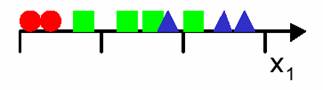
Figure 5.1: 3-class pattern recognition problem in one-dimension.

  

After doing this, we notice that there exists too much overlap among the classes, so we decide to incorporate a second feature to try and improve separability. We decide to preserve the granularity of each axis, which raises the number of bins from 3 in one-dimension, to 3²=9 in two-dimensions (Figure 5.2). At this point we need to make a decision: do we maintain the density of examples per bin or do we keep the number of examples had for the one-dimensional case? Choosing to maintain the density increases the number of examples from 9 in one-dimension to 27 two-dimensions (Figure 5.2a). Choosing to maintain the number of examples results in a two-dimensional scatter plot that is very sparse (Figure 5.2b).

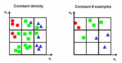
                                               (a)                                                     (b)     

Figure 5.2: The results of decisions made after preserving the granurality of each axis, a. the density of examples are maintained, and thus the number of examples are increased, and b. the number of examples are maintained resulting sparse scatter plot.

Moving to three features makes the problem worse. The number of bins grows to 3³=27. For the same density of examples the number of needed examples becomes 81. For the same number of examples, the 3D scatter plot is almost empty (Figure 5.3).

 

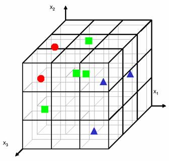
Figure 5.3: 3-class pattern recognition problem increased into three-dimensions.

  

Obviously, our approach to divide the sample space into equally spaced bins was quite inefficient. There are other approaches that are much less susceptible to the curse of dimensionality, but the problem still exists. How do we beat the curse of dimensionality? By incorporating prior knowledge, by providing increasing smoothness of the target function, and by reducing the dimensionality. In practice, the curse of dimensionality means that, for a given sample size, there is a maximum number of features above which the performance of our classifier will degrade rather than improve (Figure 5.4). In most cases, the additional information that is lost by discarding some features is more than compensated by a more accurate mapping in the lower dimensional space.

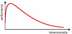
Figure 5.4: The dimensionality and performance relation in pattern recognition.

 

There are many implications of the curse of dimensionality. Exponential growth in the number of examples required to maintain a given sampling density, that is, for a density of N examples/bin and D dimensions, the total number of examples is N^D. Exponential growth in the complexity of the target function ( a density estimate) with increasing dimensionality. A function defined in high-dimensional space is likely to be much more complex than a function defined in a lower-dimensional space, and those complications are harder to discern. This means that, in order to learn it well, a more complex target function requires denser sample points. What to do if it ain’t Gaussian? For one dimension a large number of density functions can be found in textbooks, but for high-dimensions only the multivariate Gaussian density is available. Moreover, for larger values of D the Gaussian density can only be handled in a simplified form. Humans have an extraordinary capacity to discern patterns and clusters in 1, 2 and 3-dimensions, but these capabilities degrade drastically for 4 or higher dimensions.

Two approaches are available to perform dimensionality reduction: feature extraction, that is creating a subset of new features by combinations of the existing features, and feature selection, which is choosing a subset of all the features ( the ones more informative)

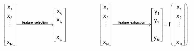
Figure 5.5: The approaches for reducing dimensionality.

  

The problem of feature extraction can be stated as given a feature space x_i Î R^N find a mapping y=f(x): R^N®R^M with M<N such that the transformed feature vector y_i Î R^M preserves (most of) the information or structure in R^N. An optimal mapping y=f(x) will be one that results in no increase in the minimum probability of error. This is, a Bayes decision rule applied to the initial space R^N and to the reduced space R^M yield the same classification rate.

In general, the optimal mapping y=f(x) will be a non-linear function. However, there is no systematic way to generate non-linear transforms. The selection of a particular subset of transforms is problem dependent. For this reason, feature extraction is commonly limited to linear transforms: y=Wx (Figure 5.6), this is, y is a linear projection of x. Note that, when the mapping is a non-linear function, the reduced space is called a manifold. We will focus on linear feature extraction for now.

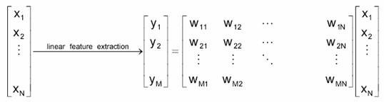
Figure 5.6: The approaches for reducing dimensionality.

  

The selection of the feature extraction mapping y=f(x) is guided by an objective function that we seek to maximize (or minimize). Depending on the criteria used by the objective function, feature extraction techniques are grouped into two categories: Signal representation where the goal of the feature extraction mapping is to represent the samples accurately in a lower-dimensional space, and Classification where the goal of the feature extraction mapping is to enhance the class-discriminatory information in the lower-dimensional space. Within the realm of linear feature extraction, two techniques are commonly used. Principal Components Analysis (PCA) uses a signal representation criterion, while Linear Discriminant Analysis (LDA) uses a signal classification criterion. The objective of PCA is to perform dimensionality reduction while preserving as much of the randomness (variance) in the high-dimensional space as possible.

We begin by considering the problem of representing all of the vectors in a set of n dimensional samples x₁,…,x_n by a single vector x₀. To be more specific, suppose that we want to find a vector x₀ such that the sum of the squared distances between x₀ and the various x_k is as small as possible. We define the squared-error criterion function J₀(x₀) by

                                                                                                      (5.1)

and seek the value of x₀ that minimizes J₀. The solution to this problem is given by x₀ = m, where m is the sample mean,

                                                                                                                        (5.2)

This can be easily verified by writing

                                                      

      

                                                                                 (5.3)

Since the second sum is independent of x₀, this expression is obviously minimized by the choice x₀ =m.

The sample mean is a zero-dimensional representation of the data set. It is sim­ple, but it does not reveal any of the variability in the data. We can obtain a more interesting, one-dimensional representation by projecting the data onto a line run­ning through the sample mean. Let e be a unit vector in the direction of the line. Then the equation of the line can be written as

x= m + ae,                                                                                                                          (5.4)

where the scalar a (which takes on any real value) corresponds to the distance of any point x from the mean m. If we represent x_k by m+a_ke, we can find an optimal set of coefficients a_k by minimizing the squared-error criterion function

                                             (5.5)

Recognizing that , partially differentiating with respect to a_k, and setting the derivative to zero, we obtain    I

                                                                                                               (5.6)

Geometrically, this result merely says that we obtain a least squares solution by projecting the vector x_k onto the line in the direction of e that passes through the sample mean.

This brings us to the more interesting problem of finding the best direction e for the line. The solution to this problem involves the so-called scatter matrix S defined by

                                                                                                  (5.7)

The scatter matrix should look familiar-it is merely n-1 times the sample covariance matrix. It arises here when we substitute a_k found in Eq. 5.5 into Eq. 5.6 to obtain

                                                                                              (5.8)

Clearly, the vector e that minimizes J₁ also maximizes . We use the method of Lagrange multipliers to maximize subject to the constraint that . Letting l be the undetermined multiplier, we differentiate

                                                                                                          (5.9)

with respect to e to obtain

                                                                                                                  (5.10)

Setting this gradient vector equal to zero, we see that e must be an eigenvector of the scatter matrix:

                                                                                                                              (5.11)

In particular, because ==, it follows that to maximize , we want to select the eigenvector corresponding to the largest eigenvalue of the scatter matrix. In other words, to find the best one-dimensional projection of the data (best in the least sum-of-squared-error sense), we project the data onto a line through the sample mean in the direction of the eigenvector of the scatter matrix having the largest eigenvalue.

This result can be readily extended from a one-dimensional projection to a dimensional projection. In place of eq.5.4, we write

                                                                                                                  (5.12)

where d’ <d. It is not difficult to show that the criterion function

                                                                                          (5.13)

is minimized when the vectors e₁…..e_d’ are the d’ eigenvectors of the scatter ma­trix having the largest eigenvalues. Because the scatter matrix is real and symmetric, these eigenvectors are orthogonal. They form a natural set of basis vectors for repre­senting any feature vector x. The coefficients a_i in eq.5.12 are the components of x in that basis, and are called the principal components. Geometrically, if we picture the data points x₁…x_n as forming a d-dimensional, hyperellipsoidally shaped cloud. Then the eigenvectors of the scatter matrix are the principal axes of that hyperellip­soid. Principal component analysis reduces the dimensionality of feature space by restricting attention to those directions along which the scatter of the cloud is great­est.

PCA dimensionality reduction can be summarized as folllows. The optimal approximation of a random vector x ÎR^N by a linear combination of M (M<N) independent vectors is obtained by projecting the random vector x onto the eigenvectors corresponding to the largest eigenvalues of the covariance matrix.

 

5.3 Principal Component Analysis in MATLAB (prepca, trapca)

  

In situations, where the dimension of the input vector is large, but the components of the vectors are highly correlated (redundant), it is useful to reduce the dimension of the input vectors. An effective procedure for performing this operation is principal component analysis. This technique has three effects:

·     it orthogonalizes the components of the input vectors (so that they are uncorrelated with each other);

·     it orders the resulting orthogonal components (principal components) so that those with the largest variation come first; and

·     it eliminates those components that contribute the least to the variation in the data set. The following code illustrates the use of prepca, which performs a principal component analysis.

[pn,meanp,stdp] = prestd(p);

[ptrans,transMat] = prepca(pn,0.02);

  

  

  

  

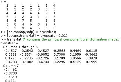
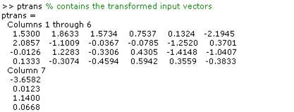
Note that we first normalize the input vectors, using prestd, so that they have zero mean and unity variance. This is a standard procedure when using principal components. In this example, the second argument passed to prepca is 0.02. This means that prepca eliminates those principal components that contribute less than 2% to the total variation in the data set. The matrix ptrans contains the transformed input vectors. The matrix transMat contains the principal component transformation matrix. After the network has been trained, this matrix should be used to transform any future inputs that are applied to the network. It effectively becomes a part of the network, just like the network weights and biases. If you multiply the normalized input vectors pn by the transformation matrix transMat, you obtain the transformed input vectors ptrans. If prepca is used to preprocess the training set data, then whenever the trained network is used with new inputs they should be preprocessed with the transformation matrix that was computed for the training set. This can be accomplished with the routine trapca. In the following code, we apply a new set of inputs to a network we have already trained.

 

pnewn = trastd(pnew,meanp,stdp);

pnewtrans = trapca(pnewn,transMat);

a = sim(net,pnewtrans);

 

5.4 Sample PCA Application in MATLAB

In this example, we take a simple set of 2-D data and apply PCA to determine the principal axes. Although the technique is used with many dimensions, two-dimensional data will make it simpler to visualise. First, we generate a set of data for analysis (Figure 5.7).

The Principal Component Analysis is then performed. First, the covariance matrix is calculated:

From this the principal components are calculated:

  

Figure 5.7: The sample dataset used in sample application.

  

Figure 5.8: The principal components of the dataset.

  

The red line in Figure 5.8 represents the direction of the first principal component and the green is the second. Note how the first principal component lies along the line of greatest variation, and the second lies perpendicular to it. Where there are more than two dimensions, the second component will be both perpendicular to the first, and along the line of next greatest variation.

By multiplying the original dataset by the principal components, the data is rotated so that the principal components lie along the axes:

Figure 5.9: The principal components that are rotated.

  

The most common use for PCA is to reduce the dimensionality of the data while retaining the most information.

The source code for the sample application can be found in pca1.m.

 

REFERENCES

  

[1]        Duda, R.O., Hart, P.E., and Stork D.G., (2001). Pattern Classification. (2^nd ed.). New York: Wiley-Interscience Publication.

[2]        Neural Network Toolbox For Use With MATLAB, User’s Guide, (2003) Mathworks Inc., ver.4.0

[3]        Gutierrez-Osuna R., Introduction to Pattern Analysis, Course Notes, Department of Computer Science, A&M University, (http://research.cs.tamu.edu/prism/lectures/pr/pr_l1.pdf ), Texas