Chapter 4 Bayesian Decision Theory
4.1 Introduction
Bayesian decision theory is a fundamental statistical approach to the problem of pattern classification. It is considered the ideal case in which the probability structure underlying the categories is known perfectly. While this sort of stiuation rarely occurs in practice, it permits us to determine the optimal (Bayes) classifier against which we can compare all other classifiers. Moreover, in some problems it enables us to predict the error we will get when we generalize to novel patterns.
This approach is based on quantifying the tradeoffs between various classification decisions using probability and the costs that accompany such decisions. It makes the assumption that the decision problem is posed in probabilistic terms, and that all of the relevant probability values are known.
Let us reconsider the hypothetical problem posed in Chapter 1 of designing a classifier to separate two kinds of fish: sea bass and salmon. Suppose that an observer watching fish arrive along the conveyor belt finds it hard to predict what type will emerge next and that the sequence of types of fish appears to be random. In decision-theoretic terminology we would say that as each fish emerges nature is in one or the other of the two possible states: Either the fish is a sea bass or the fish is a salmon. We let w denote the state of nature, with w = w1 for sea bass and w = w2 for salmon. Because the state of nature is so unpredictable, we consider w to be a variable that must be described probahilistically.

Figure 4.1: Class conditional density functions show the probabiltiy density of measuring a particular feature value x given the pattern is in category wi.
If the catch produced as much sea bass as salmon, we would say that the next fish is equally likely to be sea bass or salmon. More generally, we assume that there is some prior probability P(w1) that the next fish is sea bass, and some prior probability P(w2) that it is salmon. If we assume there are no other types of fish relevant here, then P(w1)+ P(w2)=1. These prior probabilities reflect our prior knowledge of how likely we are to get a sea bass or salmon before the fish actually appears.
If we are forced to make a decision about the type of fish that will appear next just by using the value of the prior probahilities we will decide w1 if P(w1)> P(w2) otherwise decide w2. This rule makes sense if we are to judge just one fish, but if we were to judge many fish, using this rule repeatedly, we would always make the same decision even though we know that both types of fish will appear. Thus, it does not work well depending upon the values of the prior probabilities.
In most circumstances, we are not asked to make decisions with so little information. We might for instance use a lightness measurement x to improve our classifier. Different fish will yield different lightness readings, and we express this variability: we consider x to be a continuous random variable whose distribution depends on the state of nature and is expressed as p(x|w). This is the class-conditional probability density (state-conditional probability density) function, the probability density function for x given that the state of nature is in w. Then the difference between p(x|w1) and p(x|w2) describes the difference in lightness between populations of sea bass and salmon (Figure 4.1).
Suppose that we know both the prior probabilities P(wj) and the conditional densities p(x|wj) for j = 1, 2. Suppose further that we measure the lightness of a fish and discover that its value is x. How does this measurement influence our attitude concerning the true state of nature? We note first that the (joint) probability density of finding a pattern that is in category wj and has feature value x can be written in two ways: p(wj,x) = P(wj|x) p(x) = p(x|wj) P(wj). Rearranging these leads us to the answer to our question, which is called Bayes formula:
![]() (4.1)
(4.1)
where in this case of two categories
![]() (4.2)
(4.2)
Bayes formula can be expressed informally as
![]() (4.3)
(4.3)
Bayes formula shows that by observing the value of x we can convert the prior probability P(wj) to the posterior probability P(wj|x) -the probability of the state of nature being wj given that feature value x has been measured. p(x|wj) is called the likelihood of wj with respect to x, a term chosen to indicate that, other things being equal, the category wj, for which p(x|wj) is large is more “likely” to be the true category. Notice that it is the product of the likelihood and the prior probability that is most important in determining the posterior probability; the evidence factor p(x), can be viewed as a scale factor that guarantees that the posterior probabilities sum to one. The variation of posterior probability P(wj|x) with x is illustrated in Figure 4.2 for the case P(w1)=2/3 and P(w2)=1/3.
If we have an observation x for which P(w1|x)>P(w2|x), we would naturally be inclined to decide that the true state of nature is w1. The probability of error is calculated as
![]() (4.4)
(4.4)
The Bayes decision rule is stated as
Decide w1 if P(w1|x)>P(w2|x); otherwise decide w2 (4.5)
Under this rule eq.4.4 becomes
Figure 4.2: Posterior probabilities.
P(error|x)=min[P(w1|x), P(w2|x)] (4.6)
This form of decision rule emphasizes the role of the posterior probabilities. As being equivalent, the same rule can be expressed in terms of conditional and prior probabilities as:
Decide w1 if p(x|w1)P(w1) > p(x|w2)P(w2); otherwise decide w2 (4.7)
4.2 Bayesian Decision Theory (continuous)
We shall now formalize the ideas just considered, and generalize them in four ways: by allowing the use of more than one feature, by allowing more than two states of nature, by allowing actions other than merely deciding the state of nature, and by introducing a loss function more general than the probability of error. Allowing the use of more than one feature merely requires replacing the scalar x by the feature vector x, where x is in a d-dimensional Euclidean space Rd called the feature space. Allowing more than two states of nature provides us with a useful generalization for a small notational expense as {w1… wc}. Allowing actions other than classification as {a1…aa} allows the possibility of rejection-that is, of refusing to make a decision in close (costly) cases. The loss function states exactly how costly each action is, and is used to convert a probability determination into a decision. Cost functions let us treat situations in which some kinds of classification mistakes are more costly than others. Then the posterior probability can be computed by Bayes formula as:
![]() (4.8)
(4.8)
where the evidence is now
![]() (4.9)
(4.9)
Suppose that we observe a particular x and that we contemplate taking action ai. If the true state of nature is wj by definition, we will incur the loss l(ai|wj). Because P(wj|x) is the probability that the true state of nature is wj, the expected loss associated with taking action ai is
![]() (4.10)
(4.10)
An expected loss is called a risk, and R(ai|x) is called the conditional risk. Whenever we encounter a particular observation x, we can minimize our expected loss by selecting the action that minimizes the conditional risk.
If a general decision rule a(x) tells us which action to take for every possible observation x, the overall risk R is given by
![]() (4.11)
(4.11)
Thus, the Bayes decision rule states that to minimize the overall risk, compute the conditional risk given in Eq.4.10 for i=1…a and then select the action ai for which R(ai|x) is minimum. The resulting minimum overall risk is called the Bayes risk, denoted R, and is the best performance that can be achieved.
4.2.1 Two-Category Classification
When these results are applied to the special case of two-category classification problems, action a1 corresponds to deciding that the true state of nature is w1, and action a2 corresponds to deciding that it is w2. For notational simplicity, let lij=l(ai|wj) be the loss incurred for deciding wi, when the true state of nature is wj. If we write out the conditional risk given by Eq.4.10, we obtain
![]() (4.12)
(4.12)
![]() (4.13)
(4.13)
There are a variety of ways of expressing the minimum-risk decision rule, each having its own minor advantages. The fundamental rule is to decide w1 if R(a1|x)<R(a2|x). In terms of the posterior probabilities, we decide w1 if
R(a1|x)<R(a2|x)
![]()
![]() (4.14)
(4.14)
or in terms of the prior probabilities
![]() (4.15)
(4.15)
or alternatively as likelihood ratio
![]() (4.16)
(4.16)
This form of the decision rule focuses on the x-dependence of the probability densities. We can consider p(x|wj) a function of wj (i.e., the likelihood function) and then form the likelihood ratio p(x|w1)/ p(x|w2). Thus the Bayes decision rule can be interpreted as calling for deciding w1 if the likelihood ratio exceeds a threshold value that is independent of the observation x.
4.3 Minimum Error Rate Classification
In classification problems, each state of nature is associated with a different one of the classes, and the action ai is usually interpreted as the decision that the true state of nature is wi. If action ai is taken and the true state of nature is wj then the decision is correct if i=j and in error if i¹j. If errors are to be avoided it is natural to seek a decision rule, that minimizes the probability of error, that is the error rate.
This loss function is so called symetrical or zero-one loss function is given as
![]() (4.17)
(4.17)
This loss function assigns no loss to a correct decision, and assigns a unit loss to any error: thus, all errors are equally costly. The risk corresponding to this loss function is precisely the average probability of error because the conditional risk for the two-category classification is
![]()
![]()
![]() (4.18)
(4.18)
and P(wj|x) is the conditional probability that action ai is correct. The Bayes decision rule to minimize risk calls for selecting the action that minimizes the conditional risk. Thus, to minimize the average probability of error, we should select the i that maximizes the posterior probability P(wj|x). In other words, for minimum error rate:
Decide wi if P(wi|x)>P(wj|x) for all i¹j (4.19)
This is the same rule as in Eq.4.5. The region in the input space where we decide w1 is denoted R1.
We saw in Figure 4.1 some class-conditional probability densities and the posterior probabilities: Figure 4.3 shows the likelihood ratio for the same case. The threshold value qa marked is from the same prior probabilities but with a zero-one loss function. If we penalize mistakes in classifying w1 patterns as w2 more than the converse then Eq.4.14 leads to the threshold qb marked.
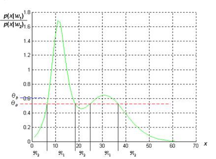
Figure 4.3: The likelihood ratio p(x|w1)/p(x|w2) for the distributions shown in Figure 4.1. If we employ a zero-one or classification loss, our decision boundaries are determined by the threshold, if our loss function penalizes miscategorizing w2 as w1 patterns more than the converse, we get the larger threshold, and hence R1 becomes smaller.
4.3.1 Minimax Criterion
In-order to design a classifier to perform well over a range of prior probabilities the worst overall risk for any value of the priors is as small as possible that is, minimize the maximum possible overall risk. Let R1 denote that (as yet unknown) region in feature space where the classifier decides w1 and likewise for R2 and w2, and then we write our overall risk Eq.4.11 in terms of conditional risks:
![]()
![]()
By using the fact
that P(w2)=1- P(w1)
and that ![]() the
function above can be rewritten the risk as:
the
function above can be rewritten the risk as:
 (4.20)
For minimax solution, the following condition should be satisfied.
![]() (4.21)
(4.21)
and
![]() (4.22)
(4.22)
in Eq.4.20 is known as minimax risk.
If we can find a boundary such that the constant of proportionality is 0, then the risk is independent of priors. This is the minimax risk, Rmm
![]() (4.23)
(4.23)
4.4 The Gaussian (Normal) Density
The definition of the expected value of a scalar function f(x) defined for some density p(x) is given by
![]() (4.24)
(4.24)
If the values of the feature x are restricted to points in a discrete set D we must sum over all samples as
![]() (4.25)
(4.25)
where P(x) is the probability mass.
The continuous univariate normal density is given by
![]() (4.26)
(4.26)
where mean m (expected value, average) is given by
![]() (4.27)
(4.27)
and the special expectation that is variance (squared deviation) is given by
![]() (4.28)
(4.28)
The univariate normal density is specified by its two parameters, its mean m, and the variance s. Samples from normal distributions tend to cluster about the mean, and the extend to which they spread out depends on the variance (Figure 4.4).
The multivariate normal density in d dimensions is written as
 (4.29)
where x is a d-component column vector, m is the d-component mean vector, S is d´d covariance matrix, |S| is its determinant and S-1 is its inverse and mean vector m becomes
Figure 4.4: A univariate Gaussian distribution has roughly 95% of its area in the range | x-m | £ 2s.
 (4.30)
The covariance matrix S is defined as the square matrix whose ijth element sij is the covariance of xi and xj: The covariance of two features measures their tendency to vary together, i.e., to co-vary.
![]() (4.31)
(4.31)
where i, j=1,…,d. Therefore, in expanded form we have


 (4.32)
We can use vector
product ![]() to
write the covariance matrix as
to
write the covariance matrix as
![]() (4.33)
(4.33)
Thus S is
symmetric, and its diagonal elements are the variances of the respective
individual elements xi of x (e.g.,![]() ), which can never be
negative; the off-diagonal elements are the covariances of xi
and xj, which can be positive or negative. If the variables xi
and xj are statistically independent, the covariances
), which can never be
negative; the off-diagonal elements are the covariances of xi
and xj, which can be positive or negative. If the variables xi
and xj are statistically independent, the covariances ![]() are zero, and the
covariance matrix is diagonal. If all the off-diagonal elements are zero, p(x)
reduces to the product of the univariate normal densities for the components of
x. The analog to the Cauchy-Schwarz inequality comes from recognizing
that if w is any d-dimensional vector, then the variance of wTx
can never be negative. This leads to the requirement that the quadratic
form wTSw never be negative. Matrices for which
this is true are said to be positive semidefinite; thus, the covariance
matrix is positive semidefinite.
are zero, and the
covariance matrix is diagonal. If all the off-diagonal elements are zero, p(x)
reduces to the product of the univariate normal densities for the components of
x. The analog to the Cauchy-Schwarz inequality comes from recognizing
that if w is any d-dimensional vector, then the variance of wTx
can never be negative. This leads to the requirement that the quadratic
form wTSw never be negative. Matrices for which
this is true are said to be positive semidefinite; thus, the covariance
matrix is positive semidefinite.
Linear combinations of jointly normally distributed random variables, independent or not, are normally distributed.
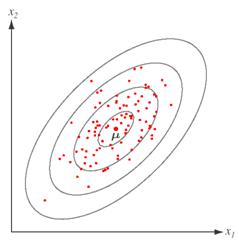
Figure 4.5: Samples drawn from a two-dimensional Gaussian lie in a cloud centered on the mean. The ellipses show lines of equal probability density of the Gaussian.
Figure 4.6: The contour lines show the regions for which the function has constant density. From the equation for the normal density, it is apparent that points, which have the same density, must have the same constant term (x -µ)-1S(x -µ).
As with the univariate density, samples from a normal population tend to fall in a single cloud or cluster centered about the mean vector, and the shape of the cluster depends on the covariance matrix (see Figure 4.5 and Figure 4.6).
From the multivariate normal density formula in Eq.4.27 notice that the density is constant on surfaces where the squared distance (Mahalanobis distance)(x -µ)TS-1(x -µ) is constant. These paths are called contours (hyperellipsoids). The principle axes of these contours are given by the eigenvectors of S, where the eigenvalues determine the lengths of these axes.
The covariance matrix for 2 features x and y is diagonal (which implies that the 2 features don't co-vary), but feature x varies more than feature y. The contour lines are stretched out in the x direction to reflect the fact that the distance spreads out at a lower rate in the x direction than it does in the y direction. The reason that the distance decreases slower in the x direction is because the variance for x is greater and thus a point that is far away in the x direction is not quite as distant from the mean as a point that is far away in the y direction (see Figure 4.9).
4.4.1 Interpretation of eigenvalues and eigenvectors
It is sometimes convenient to perform a coordinate transformation that converts an arbitrary multivariate normal distribution into a spherical one –that is, one having a covariance matrix proportional to the identity matrix I. If we define F to be the matrix whose columns are the orthonormal eigenvectors of S, and L the diagonal matrix of the corresponding eigenvalues, then the transformation A=FL-1/2 applied to the coordinates ensures that the transformed distribution has covariance matrix equal to the identity matrix I. If we view matrix A as a linear transformation, an eigenvector represents an invariant direction in the vector space. When transformed by A, any point lying on the direction defined by v will remain on that direction, and its magnitude will be multipled by the corresponding eigenvalue (see Figure 4.7).
Figure 4.7: The linear transformation of a matrix.
Given the covariance matrix S of a Gaussian distribution, the eigenvectors of S are the principal directions of the distribution, and the eigenvalues are the variances of the corresponding principal directions. The linear transformation defined by the eigenvectors of S leads to vectors that are uncorrelated regardless of the form of the distribution. If the distribution happens to be Gaussian, then the transformed vectors will be statistically independent.

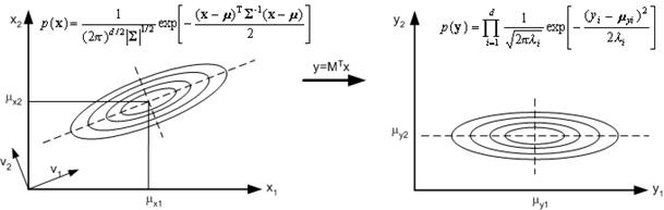
Figure 4.8: The linear transformation.

Figure 4.9: The covariance matrix for two features x and y do not co-vary, but feature x varies more than feature y.
The covariance matrix for two features x and y is diagonal, and x and y have the exact same variance. This results in euclidean distance contour lines (see Figure 4.10).
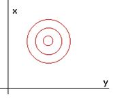
Figure 4.10: The covariance matrix for two features that have exact same variances.
The covariance matrix is not diagonal. Instead, x and y have the same variance, but x varies with y in the sense that x and y tend to increase together. So the covariance matrix would have identical diagonal elements, but the off-diagonal element would be a strictly positive number representing the covariance of x and y (see Figure 4.11).
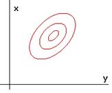
Figure 4.11: The covariance matrix for two features that has exact same variances, but x varies with y in the sense that x and y tend to increase together.
4.5 Discriminant Functions, and Decision Surfaces
There are many different ways to represent pattern classifiers. One of the most useful is in terms of a set of discriminant functions gi(x), i=1,…,c. The classifier is said to assign a feature vector x to class wi if
gi(x) > gj(x), i¹j (4.34)
A Bayes classifier is easily and naturally represented in this way. For the general case with risks, we can let gi(x)= - R(ai|x), because the maximum discriminant function will then correspond to the minimum conditional risk. For the minimum error-rate case, we can simplify things further by taking gi(x)= P(wi|x), so that the maximum discriminant function corresponds to the maximum posterior probability. Clearly, the choice of discriminant functions is not unique. In particular, for minimum-error rate classification, any of the following choices gives identical classification results, but some can be much simpler to understand or to compute than others:
 (4.35)
![]() (4.36)
(4.36)
![]() (4.37)
(4.37)
Even though the discriminant functions can be written in a variety of forms, the decision rules are equivalent. The effect of any decision rule is to divide the feature space into c decision boundaries, R1,…, Rc. If gi(x) > gj(x) for all i¹j, then x is in Ri, and the decision rule calls for us to assign x to wi. The regions are separated by decision boundaries, surfaces in feature space where ties occur among the largest discriminant functions.
While the two-category case is just a special instance of the multicategory case, instead of using two discriminant functions g1 and g2 and assigning x to w1 if g1>g2, it can be treated by using a single discriminant function
![]() (4.38)
(4.38)
and to use the following decision rule: Decide w1 if g(x)>0; otherwise decide w2. One of the various forms in which the minimum-error rate discriminant function can be written, the following two are particularly convenient:
![]() (4.39)
(4.39)
![]() (4.40)
(4.40)
4.6 Discriminant Functions For The Normal Density
Eq.4.37 can be easily evaluated if the densities are multivariate normal. In this case, from eq.4.29 we have
![]() (4.41)
(4.41)
Case 1: ![]()
The simplest case occurs when the features that are measured is independent of each other, that is, statistically independent, and when each feature has the same variance, s2. For example, if we were trying to recognize an apple from an orange, and we measured the colour and the weight as our feature vector, then chances are that there is no relationship between these two properties. The non-diagonal elements of the covariance matrix are the covariances of the two features x1=colour and x2=weight. But because these features are independent, their covariances would be 0. Therefore, the covariance matrix for both classes would be diagonal, being merely s2 times the identity matrix I.
As a second simplification, assume that the variance of colours is the same is the variance of weights. This means that there is the same degree of spreading out from the mean of colours as there is from the mean of weights. If this is true for some class i then the covariance matrix for that class will have identical diagonal elements. Finally, suppose that the variance for the colour and weight features is the same in both classes. This means that the degree of spreading for these two features is independent of the class from which you draw your samples. If this is true, then the covariance matrices will be identical. When normal distributions are plotted that have a diagonal covariance matrix that is just a constant multplied by the identity matrix, their cluster points about the mean are shperical in shape.
Geometrically, this corresponds to the situation in which the samples fall in equal-size hyperspherical clusters, the cluster for the ith class being centered about the mean vector mi (see Figure 4.12). The computation of the determinant and the inverse of Si is particularly easy:
![]() and
and
![]() (4.42)
(4.42)
Because both |Si| and the (d/2) ln 2p term in Eq.4.41 are independent of i, they are unimportant additive constants that can be ignored. Thus, we obtain the simple discriminant functions
![]()
![]()
![]()
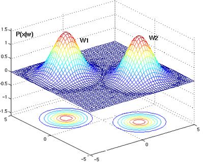
Figure 4.12: Since the bivariate normal densities have diagonal covariance matrices, their contours are spherical in shape. Each class has the exact same covariance matrix, the circular lines forming the contours are the same size for both classes. This is because identical covariance matrices imply that the two classes have identically shaped clusters about their mean vectors.
![]() (4.43)
(4.43)
where
![]() (4.44)
(4.44)
If the prior probabilities are not equal,
then Eq.4.43 shows that the squared distance ![]() must be normalized by
the variance
must be normalized by
the variance ![]() and offset by
adding ln P(wi); thus, if x is
equally near two different mean vectors, the optimal decision will favor the a
priori more likely category.
and offset by
adding ln P(wi); thus, if x is
equally near two different mean vectors, the optimal decision will favor the a
priori more likely category.
Regardless of whether the prior
probabilities are equal or not, it is not actually necessary to compute
distances. Expansion of the quadratic form ![]() yields
yields
![]() (4.45)
(4.45)
which appears to be a quadratic function of x. However, the quadratic term xTx is the same for all i, making it an ignorable additive constant. Thus, we obtain the equivalent linear discriminant functions
![]() (4.46)
(4.46)
where
![]() (4.47)
(4.47)
and
![]() (4.48)
(4.48)
We call wi0 the threshold or bias for the ith category.
The decision boundaries for these discriminant functions are found by intersecting the functions gi(x) and gj(x) where i and j represent the 2 classes with the highest a posteriori probabilites. As in the univariate case, this is equivalent to determining the region for which gi(x) is the maximum of all the discriminant functions. By setting gi(x) = gj(x) we have that:
![]() (4.49)
(4.49)
Consider the term wi0 - wj0:
![]()
![]()

 (4.50)
Now, by adding and subtracting the same term, we get:

 (4.51)
By letting:
 (4.52)
the result is:
 (4.53)
But because of the way we define wi
and wj, this is just:
![]() (4.54)
(4.54)
So from the originial equation we have :
![]() (4.55)
(4.55)
and after multiplying through by variance the final decision boundary is given by:
![]() (4.56)
(4.56)
Now let w =![]() . Then this boundary can be written as:
. Then this boundary can be written as:
![]() (4.57)
(4.57)
where
(4.58)
and
w =![]() (4.59)
(4.59)
This is called the normal
form of the boundary equation. Geometrically, equations 4.57, 4.58, and
4.59 define a hyperplane throught the point x0 that is
orthogonal to the vector w. But since w=![]() then the hyperplane which
seperates Ri and Rj is orthogonal to the line that
links their means. If P(wi)=P(wj),
the second term on the right of Eq.4.58 vanishes, and thus the point
x0 is halfway between the means (equally divide the
distance between the 2 means, with a decision region on either side), and the
hyperplane is the perpendicular bisector of the line between the means (see Figure
4.13).
then the hyperplane which
seperates Ri and Rj is orthogonal to the line that
links their means. If P(wi)=P(wj),
the second term on the right of Eq.4.58 vanishes, and thus the point
x0 is halfway between the means (equally divide the
distance between the 2 means, with a decision region on either side), and the
hyperplane is the perpendicular bisector of the line between the means (see Figure
4.13).
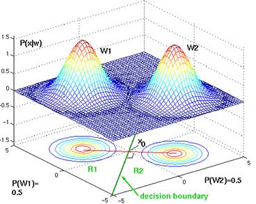
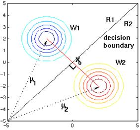
Figure 4.13: Two bivariate normal distributions, whose priors are exactly the same. Therefore, the decision bondary is exactly at the midpoint between the two means. The decision boundary is a line orthogonal to the line joining the two means.
If P(wi)¹P(wj) the point x0 shifts away from the more
likely mean. Note, however, that if the variance is small relative to the
squared distance ![]() ,
then the position of the decision boundary is relatively insensitive to the
exact values of the prior probabilities. In other words, there are 80% apples
entering the store. If you observe some feature vector of color and weight that
is just a little closer to the mean for oranges than the mean for apples,
should the observer classify the fruit as an orange? The answer depends on how
far from the apple mean the feature vector lies. In fact, if P(wi)>P(wj)
then the second term in the equation for x0 will subtract a
positive amount from the first term. This will move point x0
away from the mean for Ri. If P(wi)<P(wj)
then x0 would tend to move away from the mean for Rj. So for the above example and
using the above decision rule, the observer will classify the fruit as an
apple, simply because it's not very close to the mean for oranges, and because
we know there are 80% apples in total (see Figure 4.14 and Figure 4.15).
,
then the position of the decision boundary is relatively insensitive to the
exact values of the prior probabilities. In other words, there are 80% apples
entering the store. If you observe some feature vector of color and weight that
is just a little closer to the mean for oranges than the mean for apples,
should the observer classify the fruit as an orange? The answer depends on how
far from the apple mean the feature vector lies. In fact, if P(wi)>P(wj)
then the second term in the equation for x0 will subtract a
positive amount from the first term. This will move point x0
away from the mean for Ri. If P(wi)<P(wj)
then x0 would tend to move away from the mean for Rj. So for the above example and
using the above decision rule, the observer will classify the fruit as an
apple, simply because it's not very close to the mean for oranges, and because
we know there are 80% apples in total (see Figure 4.14 and Figure 4.15).
Figure 4.14: As the priors change, the decision boundary throught point x0 shifts away from the more common class mean (two dimensional Gaussian distributions).
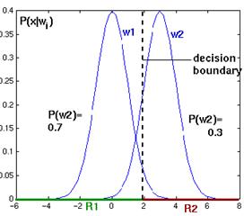

Figure 4.15: As the priors change, the decision boundary throught point x0 shifts away from the more common class mean (one dimensional Gaussian distributions).
If the prior probabilities P(wi)
are the same for all c classes, then the ln P(wi)
term becomes another unimportant additive constant that can be ignored. When
this happens, the optimum decision rule can be stated very simply: the decision
rule is based entirely on the distance from the feature vector x to the
different mean vectors. The object will be classified to Ri if it is closest to the mean
vector for that class. To classify a feature vector x, measure the
Euclidean distance ![]() from
each x to each of the c mean vectors, and assign x to the
category of the nearest mean. Such a classifier is called a minimum-distance
classifier. If each mean vector is thought of as being an ideal prototype
or template for patterns in its class, then this is essentially a template-matching
procedure.
from
each x to each of the c mean vectors, and assign x to the
category of the nearest mean. Such a classifier is called a minimum-distance
classifier. If each mean vector is thought of as being an ideal prototype
or template for patterns in its class, then this is essentially a template-matching
procedure.
Case 2: ![]()
Another simple case arises when the covariance matrices for all of the classes are identical but otherwise arbitrary. Since it is quite likely that we may not be able to measure features that are independent, this section allows for any arbitrary covariance matrix for the density of each class. In order to keep things simple, assume also that this arbitrary covariance matrix is the same for each class wi. This means that we allow for the situation where the color of fruit may covary with the weight, but the way in which it does is exactly the same for apples as it is for oranges. Instead of having shperically shaped clusters about our means, the shapes may be any type of hyperellipsoid, depending on how the features we measure relate to each other. However, the clusters of each class are of equal size and shape and are still centered about the mean for that class.
Geometrically, this corresponds to the situation in which the samples fall in hyperellipsoidal clusters of equal size and shape, the cluster for the ith class being centered about the mean vector mi. Because both Si and the (d/2) ln 2p terms in eq. 4.41 are independent of i, they can be ignored as superfluous additive constants. Using the general discriminant function for the normal density, the constant terms are removed. This simplification leaves the discriminant functions of the form:
![]()
![]() (4.60)
(4.60)
Note that, the covariance matrix no longer has a subscript i, since it is the same matrix for all classes.
If the prior probabilities P(wi) are the same for all c classes, then the ln P(wi) term can be ignored. In this case, the optimal decision rule can once again be stated very simply: To classify a feature vector x, measure the squared Mahalanobis distance (x -µi)TS-1(x -µi) from x to each of the c mean vectors, and assign x to the category of the nearest mean. As before, unequal prior probabilities bias the decision in favor of the a priori more likely category.
Expansion of the quadratic form (x -µi)TS-1(x -µi) results in a sum involving a quadratic term xTS-1x which here is independent of i. After this term is dropped from eq.4.41, the resulting discriminant functions are again linear.
After expanding out the first term in eq.4.60,
![]()
![]() (4.61)
(4.61)
![]() (4.62)
(4.62)
where
![]() (4.63)
(4.63)
and
![]() (4.64)
(4.64)
The boundary between two decision regions is given by
![]() (4.65)
(4.65)
Now examine the second term ![]() from eq.4.64. Substituting the values
for wi0 and wj0
yields:
from eq.4.64. Substituting the values
for wi0 and wj0
yields:
![]()
![]()
![]()

 (4.66)
Then, by adding and subtracting the same term:
 (4.67)
Now if we let
 (4.68)
Then the above line reduces to:
![]()
which is actually just:
![]() =0
(4.69)
=0
(4.69)
Now, starting with the original equation and substituting this line back in, the result is:
![]() =0
(4.70)
=0
(4.70)
So let
w = wi - wj
which means that the equation for the decision boundary is given by:
wTx - wTx0=0 (4.71)
Because the discriminants are linear, the resulting decision boundaries are again hyperplanes. If Ri and Rj are contiguous, the boundary between them has the equation eq.4.71 where
w = ![]() (
(![]() )
(4.72)
)
(4.72)
and
(4.73)
Again, this formula is called the normal form of the decision boundary.
As in case 1, a line through the point x0
defines this decision boundary between Ri and Rj. If the prior probabilities are
equal then x0 is halfway between the means. If the
prior probabilities are not equal, the optimal boundary hyperplane is shifted
away from the more likely mean The decision boundary is in the direction
orthogonal to the vector w = ![]() (
(![]() ); The difference lies in the fact that
the term w is no longer exactly in the direction of
); The difference lies in the fact that
the term w is no longer exactly in the direction of ![]() . Instead, the vector between mi and mj is now also multipled by the
inverse of the covariance matrix. This means that the decision boundary is no
longer orthogonal to the line joining the two mean vectors. Intstead, the boundary
line will be tilted depending on how the 2 features covary and their respective
variances (see Figure 4.19). As before, with sufficient bias the decision plane
need not lie between the two mean vectors.
. Instead, the vector between mi and mj is now also multipled by the
inverse of the covariance matrix. This means that the decision boundary is no
longer orthogonal to the line joining the two mean vectors. Intstead, the boundary
line will be tilted depending on how the 2 features covary and their respective
variances (see Figure 4.19). As before, with sufficient bias the decision plane
need not lie between the two mean vectors.
To understand how
this tilting works, suppose that the distributions for class i and class
j are bivariate normal and that the variance of feature 1 is ![]() and that of feature 2 is
and that of feature 2 is ![]() . Suppose also that the
covariance of the 2 features is 0. Finally, let the mean of class i be
at (a,b) and the mean of class j be at (c,d) where a>c and b>d for
simplicity. Then the vector w will have the form:
. Suppose also that the
covariance of the 2 features is 0. Finally, let the mean of class i be
at (a,b) and the mean of class j be at (c,d) where a>c and b>d for
simplicity. Then the vector w will have the form:
![]()
This equation can provide some insight as to how the decision boundary will be tilted in relation to the covariance matrix. Note though, that the direction of the decision boundary is orthogonal to this vector, and so the direction of the decision boundary is given by:
![]()
Now consider what
happens to the tilt of the decision boundary when the values of ![]() or
or ![]() are changed (Figure
4.16). Although the vector form of w provided shows exactly which way
the decision boudary will tilt, it does not illustrate how the contour lines
for the 2 classes are changing as the variances altered.
are changed (Figure
4.16). Although the vector form of w provided shows exactly which way
the decision boudary will tilt, it does not illustrate how the contour lines
for the 2 classes are changing as the variances altered.
Figure 4.16: As the variance of feature 2 is increased, the x term in the vector will become less negative. This means that the decision boundary will tilt vertically. Similarly, as the variance of feature 1 is increased, the y term in the vector will decrease, causing the decision boundary to become more horizontal.
Does the tilting of the decision boundary from the orthogonal direction make intuitive sense? With a little thought, it is easy to see that it does. For example, suppose that you are again classifying fruits by measuring their color and weight. Suppose that the color varies much more than the weight does. Then consider making a measurement at point P in Figure 4.17:

Figure 4.17: The discriminant function evaluated at P is smaller for class apple than it is for class orange.
In Figure 4.17, the point P is at actually closer euclideanly to the mean for the orange class. But as can be seen by the ellipsoidal contours extending from each mean, the discriminant function evaluated at P is smaller for class 'apple' than it is for class 'orange'. This is because it is much worse to be farther away in the weight direction, then it is to be far away in the color direction. Thus, the total 'distance' from P to the means must consider this. For this reason, the decision bondary is tilted.
The fact that the decision boundary is not orthogonal to the line joining the 2 means, is the only thing that seperates this situation from case 1. In both cases, the decision boundaries are straight lines that pass through the point x0. The position of x0 is effected in the exact same way by the a priori probabilities.
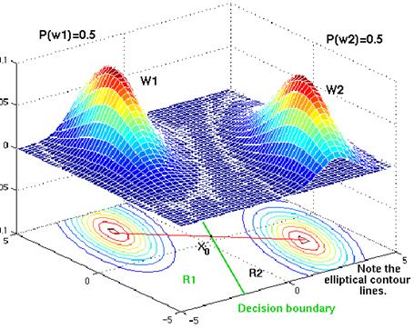
Figure 4.18: The contour lines are elliptical in shape because the covariance matrix is not diagonal. However, both densities show the same elliptical shape. The prior probabilities are the same, and so the point x0 lies halfway between the 2 means. The decision boundary is not orthogonal to the red line. Instead, it is is tilted so that its points are of equal distance to the contour lines in w1 and those in w2.
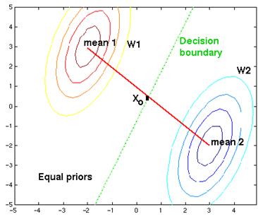
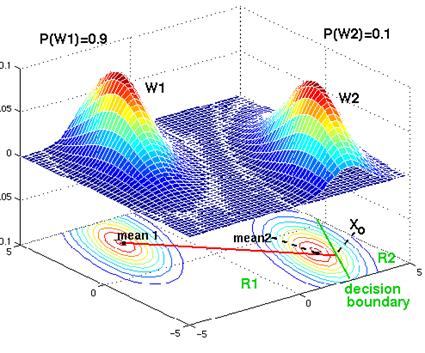
Figure 4.19: The contour lines are elliptical, but the prior probabilities are different. Although the decision boundary is a parallel line, it has been shifted away from the more likely class. With sufficient bias, the decision boundary can be shifted so that it no longer lies between the 2 means:
Case 3: ![]()
In the general multivariate normal case, the covariance matrices are different for each category. This case assumes that the covariance matrix for each class is arbitrary. The discriminant functions cannot be simplified and the only term that can be dropped from eq.4.41 is the (d/2) ln 2p term, and the resulting discriminant functions are inherently quadratic.
![]()
![]() (4.74)
(4.74)
which can equivalently be written as:
gi(x) = xTWix
+ wiTx + wi0
where
![]() and
and ![]() (4.75)
(4.75)
and
![]() (4.76)
(4.76)
Figure 4.20: Typical single-variable normal distributions showing a disconnected decision region R2
Because the expression for the gi(x) has a quadratic term in it, the decision surfaces are no longer linear. Instead, they are hyperquadratics, and they can assume any of the general forms: hyperplanes, pairs of hyperplanes, hyperspheres, hyperellipsoids, hyperparaboloids, and hyperhyperboloids of various types. The decision regions vary in their shapes and do not need to be connected. Even in one dimension, for arbitrary variance the decision regions need not be simply connected (Figure 4.20). The two-dimensional examples with different decision boundaries are shown in Figure 4.23, Figure 4.24, and in Figure 4.25.
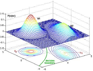
Figure 4.21: Two bivariate normals, with completely different covariance matrix, are showing a hyperquatratic decision boundary.

Figure 4.22: The contour lines and decision boundary from Figure 4.21
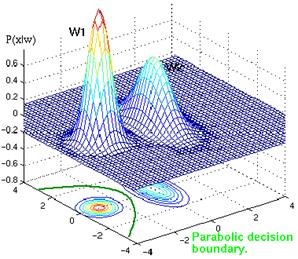
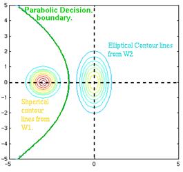
Figure 4.23: Example of parabolic decision surface.
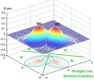
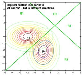
Figure 4.24: Example of straight decision surface.
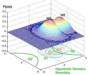

Figure 4.25: Example of hyperbolic decision surface.
4.7 Bayesian Decision Theory (discrete)
In many practical applications, instead of
assuming vector x as any point in a d-dimensional Euclidean
space, the components of x are binary valued integers, so that x can
assume only one of m discrete values v1,…,vm.
In such cases, the probability density function ![]() becomes singular; integrals of the from
given by
becomes singular; integrals of the from
given by
![]() (4.77)
(4.77)
must then be replaced by corresponding sums, such as
![]() (4.78)
(4.78)
where we understand that the summation is over all values of x in the discrete distribution. Bayes formula then involves probabilities, rather than probability densities:
![]() (4.79)
(4.79)
where
![]() (4.80)
(4.80)
The definition of conditional risk is unchanged, and the fundamental Bayes decision rule remains the same: To minimize the overall risk, select the action for which is minimum. The basic rule to minimize the error rate by mazimizing the posterior probability is also unchanged as are the discriminant functions.
As an example of a classification involving discrete features, consider two categry case with x=(x1… xd), where the components xi are either 0 or 1, and with probabilities
pi=Pr[xi=1| w1] and qi=Pr[xi=1| w2] (4.81)
This is a model of a classification problem in which, each feature gives a yes/no answer about the pattern. If pi>qi, we expect the ith feature to give a yes answer when the state of nature is w1. By assuming conditional independence we can write P(x| wi) as the product of the probabilities for the components of x as:
![]() (4.82)
(4.82)
and
![]() (4.83)
(4.83)
Then the likelihood ratio is given by
 (4.84)
and the discriminant function yields
![]() (4.85)
(4.85)
The discriminant function is linear and thus can be writeen as
![]() (4.86)
(4.86)
where
![]() (4.87)
(4.87)
and
![]() (4.88)
(4.88)
REFERENCES
[1] Statistics Toolbox For Use With MATLAB, User’s Guide, (2003) Mathworks Inc., ver.4.0
[2] Prees W. H., Teukolsky S. A., Vetterling W. T., and Flannery B. P. Numerical Recipies in C: The Art Scientific Computing, User’s Guide, (2nd Ed.) Cambridge: Cambridge University Press
[3] Duda, R.O., Hart, P.E., and Stork D.G., (2001). Pattern Classification. (2nd ed.). New York: Wiley-Interscience Publication.
[4] Duda, R.O. Pattern Recognition for Human Computer Interface, Lecture Notes, web site, http://www-engr.sjsu.edu/~knapp/HCIRODPR/PR-home.htm