3.4. IMAGE INTERPOLATION AND MOTION ESTIMATION

    In signal interpolation, we reconstruct a continuous signal from samples, image interpolation has many applications, it can be used in changing the size of a digital image to improve its appearance when viewed on a display device. Consider a digital image of 64 x 64 pixels, if the display device performs zero-order hold, each individual pixel will be visible and the image will appear blocky. If the image size is increased through interpolation and resampling prior to its display, the resulting image will appear smoother and more visually pleasant. A sequence of image frames can also be interpolated along the temporal dimension. A 24 frames/sec motion picture can be converted to a 60 fields/sec NTSC signal for TV through interpolation. Temporal interpolation can also be used to improve the appearance of a slow-motion video.

Interpolation can also be used in other applications such as image coding. For example, a simple approach to bit rate reduction would be to discard some pixels or some frames and recreate them from the coded pixels and frames.

3.4.1. Spatial Interpolation

    Consider a 2-D sequence f(n₁,n₂) obtained by sampling an analog signal f_c(x,y) through an ideal A/D converter;

                                                           (3.21)

If f_c(x,y) is bandlimited and the sampling frequencies 1/T₁ and 1/T₂ are higher than the Nyquist rate, from Section 1.5  f_c(x,y) can be reconstructed from f(n₁,n₂) with an ideal D/A converter by

                                                          (3.22)

where h(x,y) is the impulse response of an ideal separable analog lowpass filter given by

                                                                               (3.23)

There are several difficulties in using (3.22) and (3.23) for image interpolation. The analog image f_c(x,y), even with an antialiasing filter, is not truly bandlimited, so aliasing occurs when f_c(x,y) is sampled. In addition, h(x,y) in (3.23) is an infinite-extent function, so evaluation of f_c(x,y) using (3.22) cannot be carried out in practice. To approximate the interpolation by (3.22) and (3.23), one approach is to use a lowpass filter h(x,y) that is spatially limited. For a spatially limited h(x,y), the summation in (3.22) has a finite number of nonzero terms. If h(x,y) is a rectangular window function given by

h(x,y) = 1       ,                                                     (3.24)

then it is called zero-order interpolation. In zero-order interpolation, f_c(x,y) is chosen as f(n₁,n₂) at the pixel closest to (x,y). Other examples of h(x,y) which are more commonly used are functions of smoother shape, such as the spatially limited Gaussian function or the windowed ideal lowpass filter.

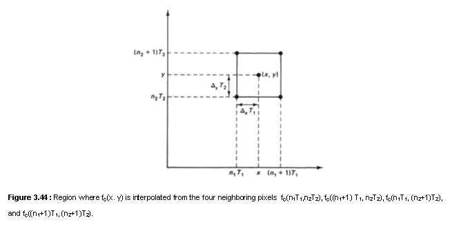
    Another simple method widely used in practice is bilinear interpolation. In this method, f_c(x,y) is evaluated by a linear combination of f(n₁,n₂) at the four closest pixels. Suppose we wish to evaluate f(x,y) for n₁T₁ £ x £ (n₁ + 1)T₁ and n₂T₂ £ y £ (n₂ +1)T₂, as shown in Figure 3.44. The interpolated f_c(x,y) in the bilinear interpolation method is

(3.25a)

where                                                                                             (3.25b)
and                                                                                                (3.25c)

Another method is polynomial interpolation. Consider a local spatial region, say 3 x 3 or 5 x 5 pixels, over which f(x,y) is approximated by a polynomial. The interpolated image  is

                                                                                                  (3.26)

where  is a term in a polynomial. An example of  when N = 6 is

=1,x,y,x²,y²,xy.                                                                                    (3.27)

The coefficients S_i can be determined by minimizing

                                             (3.28)

where y denotes the pixels over which f(x, y) is approximated. Solving (3.28) is a simple linear problem, since the are fixed. Advantages of polynomial interpolation include the smoothness of  and the simplicity of evaluating  and , partial derivatives, which are used in such applications as edge detection and motion estimation. In addition, by fitting a polynomial with fewer coefficients than the number of pixels in the region y in (3.28), some noise smoothing can be accomplished. Noise smoothing is particularly useful in applications where the partial derivatives  and  are used.

    Spatial interpolation schemes can also be developed using motion estimation algorithms discussed in the next section. One example, where an image frame that consists of two image fields is constructed from a single image field, is discussed in Section 3.4.4.

    Figure 3.45 shows an example of image interpolation. Figure 3.45(a) shows an image of 256 x 256 pixels interpolated by zero-order hold from an original image of 64 x 64 pixels. Figure 3.45(b) shows an image of 256 x 256 pixels obtained by bilinear interpolation of the same original image of 64 x 64 pixels.