3.3.3.Edge Detection by Marr and Hildreth’s Method

    In the previous two sections, we discussed edge detection algorithms that produce one edge map from an input image. Marr and Hildreth observed that significant intensity changes occur at different scales (resolution) in an image. For example, blurry shadow regions and sharply focused fine-detail

regions may be present in the same image. “Optimal” detection of significant intensity changes, therefore, generally requires the use of operators that respond to several different scales. Marr and Hildreth suggested that the original image be band-limited at several different cutoff frequencies and that an edge detection algorithm be applied to each of the images. The resulting edge maps have edges corresponding to different scales.

    Marr and Hildreth argue that edge maps of different scales contain important information about physically significant parameters. The visual world is made of elements such as contours, scratches, and shadows, which are highly localized at their own scale. This localization is also reflected in such physically important changes as reflectance change and illumination change. If the same edge is present in a set of edge maps of different scale, it represents the presence of an image intensity change due to a single physical phenomenon. If an edge is present in only one edge map, one reason may be that two independent physical phenomena are operating to produce intensity changes in the same region of the image.

    To bandlimit an image at different cutoff frequencies, the impulse response h(x,y) and frequency response H(W_x,W_y) of the lowpass filter proposed is Gaussian-shaped lowpass filter and is given by

                                                                               (3.17a)

                                                               (3.17b)

where s determines the cutoff frequency with larger s corresponding to lower cutoff frequency. The choice of Gaussian shape is motivated by the fact that it is smooth and localized in both the spatial and frequency domains. A smooth h(x,y) is less likely to introduce any changes that are not present in the original shape. A more localized h(x,y) is less likely to shift the location of edges.

    From the smoothed images, edges can be detected by using the edge detection algorithms discussed in the previous two sections. Depending on which method is used, the lowpass filtering operation in (3.17) and the partial derivative operation used for edge detection may be combined. For example, noting that Ѳ[.] and convolution * are linear, we obtain

                                                                         (3.18)

For the Gaussian function h(x,y) in (3.17), Ѳh(x,y) and its Fourier transform are given by

                                                               (3.19a)

.                                                                      (3.19b)

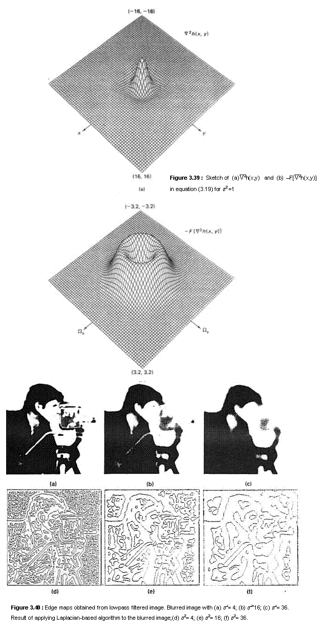
Marr and Hildreth chose, for simplicity, to detect edges by looking for zero-crossing points of Ѳf(x,y). Bandlimiting f(x,y) tends to reduce noise, thus reducing the noise sensitivity problem associated with detecting zero-crossing points. The functions Ѳf(x,y) and –F[Ѳh(x,y)] in (3.19) are sketched in Figure 3.39. Clearly, computing f(x, y)*Ѳh(x,y) is equivalent to bandpass filtering f(x,y) where s² in (3.19) is a parameter that controls the bandwidth of the bandpass filter. For a sequence f(n₁,n₂), one approach is to simply replace x and y in (3.19) with n₁ and n₂.

    Figure 3.40 shows an example of the approach under discussion. Figures 3.40(a), (b), and (c) show three images obtained by blurring the original image in Figure 3.36(a) with h(n₁,n₂) obtained by replacing x andy of h(x,y) in (3.17) with n₁ and n₂ with s² = 4, 16, and 36, respectively. Figures 3.40(d), (e), and (f) show the images obtained by detecting zero crossings of  with Ѳh(x,y) given by (3.19a) for s² = 4, 16, and 36, respectively. Marr and Hildreth used the edge maps of different scales, such as those in Figures 3.40(d), (e), and (f) for object representation in their image understanding work.