3.3.2. Laplacian-Based Methods
The objective of an edge detection algorithm is to locate the regions where the intensity is changing rapidly. In the case of a 1-D function f(x), searching for regions of rapidly changing intensity corresponds to searching for regions where f’(x) is large. For gradient-based methods, f’(x) is considered large when its magnitude |f’(x)| is greater than a threshold. Another possible way is to assume that f’(x) is large whenever it reaches a local extremum, that is, whenever the second derivative f”(x) has a zero crossing. This is illustrated in Figure 3.24. Declaring zero-crossing points as edges results in a large number of points being declared to be edge points. Since there is no check on the magnitude of f’(x). Declaring zero-crossing points as edges results in a large number of points being declared to be dege points. Since there is no check on the magnitude of f’(x), any small ripple in f(x) is enough to generate an edge point. Due to this sensitivity to noise the application of a noise reduction system prior to edge detection is very desirable in processing images with background noise.
A generalization of ![]() to
a 2-D function f(x,y) for the purpose of edge detection (see Problem 3.19) is
the Laplacian Ñ2f(x,y) given by
to
a 2-D function f(x,y) for the purpose of edge detection (see Problem 3.19) is
the Laplacian Ñ2f(x,y) given by
![]() (3.11)
(3.11)
For
a 2-D sequence f(n1,n2), the partial second derivatives ![]() and
and ![]() can be
replaced by some form of second-order differences. Second-order differences can
be represented by convolution of f(n1,n2) with the
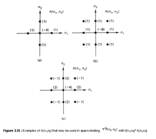
impulse response of a filter h(n1,n2). Examples of h(n1,n2)
that may be used are shown in Figure 3.35. To illustrate that f(n1,n2)*h(n1,n2)
may be viewed as a discrete approximation of Ñ2f(x, y), let us consider
h(n1,n2) in Figure 3.35(a). Suppose we approximate
can be
replaced by some form of second-order differences. Second-order differences can
be represented by convolution of f(n1,n2) with the
impulse response of a filter h(n1,n2). Examples of h(n1,n2)
that may be used are shown in Figure 3.35. To illustrate that f(n1,n2)*h(n1,n2)
may be viewed as a discrete approximation of Ñ2f(x, y), let us consider
h(n1,n2) in Figure 3.35(a). Suppose we approximate ![]() by
by
![]() (3.12)
(3.12)
We
again omitted the scaling factor, since it does not affect zero-crossing
points. Since the forward difference is used in (8.12), we can use the backward
difference in approximating ![]() :
:
![]() (3.13)
(3.13)
From (3.12) and (3.13),
![]() . (3.14)
. (3.14)
From
(3.11) and (3.14), and approximating ![]() in a similar manner, we
obtain
in a similar manner, we
obtain
![]() (3.15)
(3.15)
The
resulting ![]() is
f(n1,n2)*h(n1,n2) with h(n1,n2)
in Figure 3.35(a). Depending on how the second-order derivatives are
approximated, it is possible to derive many other impulse responses h(n1,n2),
including those shown in Figures 3.35(b) and (c).
is
f(n1,n2)*h(n1,n2) with h(n1,n2)
in Figure 3.35(a). Depending on how the second-order derivatives are
approximated, it is possible to derive many other impulse responses h(n1,n2),
including those shown in Figures 3.35(b) and (c).
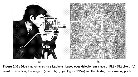
Figure 3.36 shows an example where edges were detected by looking for
zero-crossing points of ![]() . Figure 3.36(a) shows an image of 512 x
512 pixels. Figure 3.36(b) shows the zero-crossing points of
. Figure 3.36(a) shows an image of 512 x
512 pixels. Figure 3.36(b) shows the zero-crossing points of ![]() , obtained from (8.15)
and using the image in Figure 3.36(a) as f(n1,n2). Since
zero-crossing contours are boundaries between regions, they tend to be
continuous lines. As a result, edge thinning necessary in gradient-based
methods is not needed in Laplacianbased methods. In addition, algorithms that
force continuity in edge contours are not as useful in Laplacian-based methods
as in gradient-based methods. As is clear from Figure 3.33(b), however,
choosing all zero-crossing points as edges tends to generate a large number of
edge points.
, obtained from (8.15)
and using the image in Figure 3.36(a) as f(n1,n2). Since
zero-crossing contours are boundaries between regions, they tend to be
continuous lines. As a result, edge thinning necessary in gradient-based
methods is not needed in Laplacianbased methods. In addition, algorithms that
force continuity in edge contours are not as useful in Laplacian-based methods
as in gradient-based methods. As is clear from Figure 3.33(b), however,
choosing all zero-crossing points as edges tends to generate a large number of
edge points.
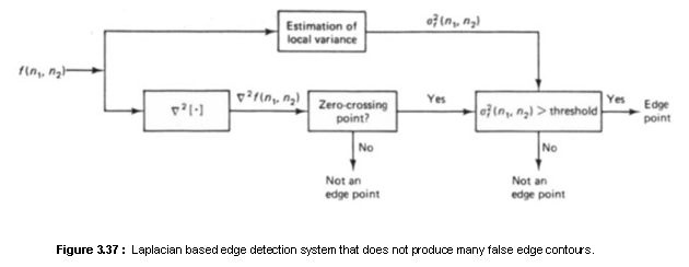
The Laplacian-based methods discussed above generate many “false” edge contours
which typically appear in regions where the local variance of the image is
small. As a special case, consider a uniform background region so that f(n1,n2)
is constant. Since ![]() is
zero and we detect edges from zero-crossing points of
is
zero and we detect edges from zero-crossing points of ![]() , any small perturbation of f(n1,n2)
is likely to cause false edge contours. One method to remove many of these
false contours is to require that the local variance is sufficiently large at
an edge point, as shown in Figure 3.34. The local variance
, any small perturbation of f(n1,n2)
is likely to cause false edge contours. One method to remove many of these
false contours is to require that the local variance is sufficiently large at
an edge point, as shown in Figure 3.34. The local variance ![]() can be estimated by
can be estimated by
 (3.16a)
where
 (3.16b)
with
M typically chosen around 2. Since ![]() is compared with a threshold, the
scaling factor 1/(2M+1)2 in (3.16a) can be eliminated. In
addition, the local variance
is compared with a threshold, the
scaling factor 1/(2M+1)2 in (3.16a) can be eliminated. In
addition, the local variance ![]() needs to be computed only for (n1,n2)
which are zero-crossing points of
needs to be computed only for (n1,n2)
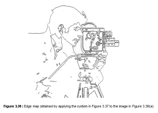
which are zero-crossing points of ![]() . Figure 3.38 shows the result of
applying the system in Figure 3.37 to the image in Figure 3.36(a). Comparison
of Figures 3.36(b) and 3.38 shows considerable reduction in the “false” edge
contours.
. Figure 3.38 shows the result of
applying the system in Figure 3.37 to the image in Figure 3.36(a). Comparison
of Figures 3.36(b) and 3.38 shows considerable reduction in the “false” edge
contours.
The system in Figure 3.34 can be interpreted as a gradient-based method. The
local variance ![]() is
closely related to the gradient magnitude. Comparing
is
closely related to the gradient magnitude. Comparing ![]() with a threshold is similar to
comparing the gradient magnitude with a threshold. Requiring that
with a threshold is similar to
comparing the gradient magnitude with a threshold. Requiring that ![]() crosses zero at an
edge can be interpreted as edge thinning. With this interpretation, we can
implement the system in Figure 3.37 by computing
crosses zero at an
edge can be interpreted as edge thinning. With this interpretation, we can
implement the system in Figure 3.37 by computing ![]() first and then by detecting the zero-crossing
points of
first and then by detecting the zero-crossing
points of ![]() only
at those points where
only
at those points where ![]() is above the chosen threshold.
is above the chosen threshold.


