3.3.1. Gradient-Based Methods
Consider an analog function f(x) which represents a typical 1-D edge, as shown in Figure 3.24(a). In typical problems, it is reasonable to consider the value x0 in the figure an edge point. One way to determine x0 is to compute the first derivative f’(x) or the second derivative f”(x). Figures 3.24(b) and (c) show f’(x) and f”(x). From the figure. the value x0 can be determined by looking for the local extremum (maximum or minimum) of f’(x) or by looking for a zero crossing of f”(x) where f”(x) changes its sign.
In addition to determining the possible edge point x0, f’(x) can also be used in estimating the strength and direction of the edge. If If’(x)I is very large, f(x) is changing very rapidly and a rapid change in intensity is indicated. If f’(x) is positive, f(x) is increasing. Based on the above observations, one approach to detecting edges is to use the system shown in Figure 3.25. In the system, first |f’(x)| is computed from f(x). If |f’(x)| is greater than some threshold, it is a candidate to be an edge. If all values of x such that |f’(x)| is greater than a certain threshold are detected to be edges, an edge will appear as a line rather than a point. To avoid this problem, we further require |f’(x)| to have a local maximum at the edge points. It may be desirable to determine whether f(x) is increasing or decreasing at x = x0. The necessary information is contained in f’(x) at x = x0. The choice of the threshold depends on the application. As the threshold increases, only the values of x where f(x) changes rapidly will be registered as candidate edges. Since it is difficult to choose the threshold optimally, some trial and error is usually involved, it is also possible to choose the threshold adaptively. The system in Figure 3.25 is based on the particular type of edge shown in Figure 3.24(a), but it is generally applicable to detecting various other types of edges.
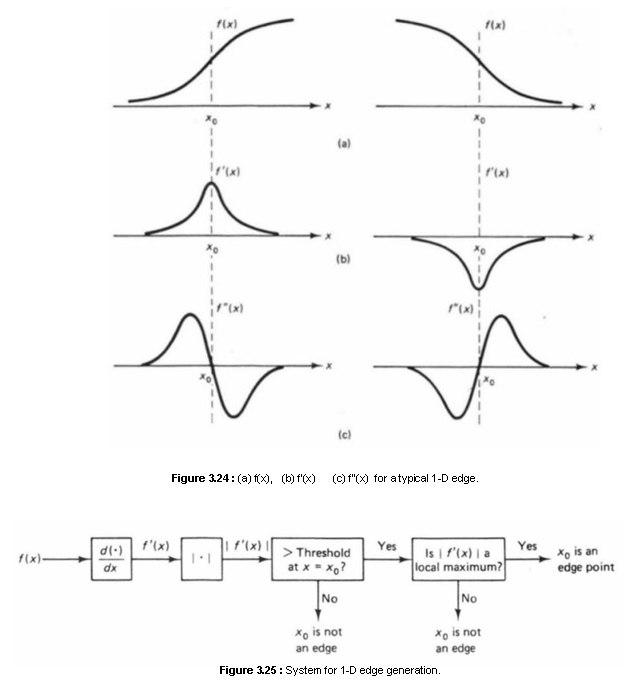
The generalization of f’(x) to a 2-D function f(x, y) is the gradient Ñf(x, y) given by
![]()
where
![]() is the unit
vector in the x-direction and
is the unit
vector in the x-direction and ![]() is the unit vector in the y-direction.
A generalization of the edge detection system Figure 3.25 based on Ñf(x,y) is shown in Figure
3.26. The magnitude of Ñf(x,y) is first computed and is then compared with a
threshold to determine candidate edge points. If all values of (x,y) such that
|Ñf(x,y)|
is greater than a certain threshold are detected to be edges, the edges will
appear as strips rather than lines. The process of determining an edge line
front a strip of candidate edge points is called edge thinning, in one simple
edge thinning algorithm, the edge points are selected by
is the unit vector in the y-direction.
A generalization of the edge detection system Figure 3.25 based on Ñf(x,y) is shown in Figure
3.26. The magnitude of Ñf(x,y) is first computed and is then compared with a
threshold to determine candidate edge points. If all values of (x,y) such that
|Ñf(x,y)|
is greater than a certain threshold are detected to be edges, the edges will
appear as strips rather than lines. The process of determining an edge line
front a strip of candidate edge points is called edge thinning, in one simple
edge thinning algorithm, the edge points are selected by
checking
if ![]() is a
local maximum in at least one direction. The property that
is a
local maximum in at least one direction. The property that ![]() achieves its local maximum in
at least one direction is usually checked along a few specified directions. In
most cases, it is sufficient to check for local maxima in only the horizontal
and vertical directions. If
achieves its local maximum in
at least one direction is usually checked along a few specified directions. In
most cases, it is sufficient to check for local maxima in only the horizontal
and vertical directions. If ![]() is a local maximum along any one of the
specified directions at a potential edge point, the potential edge point is
considered to be an edge point. One difficulty with this simple edge thinning
algorithm is that it creates a number of minor false edge lines in the vicinity
of strong edge lines. One simple method to remove most of these minor false
edge lines is to impose the following additional constraints:
is a local maximum along any one of the
specified directions at a potential edge point, the potential edge point is
considered to be an edge point. One difficulty with this simple edge thinning
algorithm is that it creates a number of minor false edge lines in the vicinity
of strong edge lines. One simple method to remove most of these minor false
edge lines is to impose the following additional constraints:
(a)If ![]() has a
local maximum at (x0,y0) in the horizontal direction but
not in the vertical direction, (x0,y0) is an edge point
when
has a
local maximum at (x0,y0) in the horizontal direction but
not in the vertical direction, (x0,y0) is an edge point
when
![]() with k typically
chosen around 2
with k typically
chosen around 2
(b)If ![]() has a local maximum at (x0,y0)
in the vertical direction but not in the horizontal direction, (x0,y0)
is an edge point when
has a local maximum at (x0,y0)
in the vertical direction but not in the horizontal direction, (x0,y0)
is an edge point when
![]() with k typically
chosen around 2
with k typically
chosen around 2
When
![]() has a local
maximum at (x0,y0) in the horizontal direction but not in
the vertical direction. Condition (a) requires that the rate of intensity
change along the horizontal direction is significantly larger than that along
the vertical direction. Condition (b) is the same as Condition (a) with the
roles of x and y reversed.
has a local
maximum at (x0,y0) in the horizontal direction but not in
the vertical direction. Condition (a) requires that the rate of intensity
change along the horizontal direction is significantly larger than that along
the vertical direction. Condition (b) is the same as Condition (a) with the
roles of x and y reversed.

An edge detection system that is based on a function such as ![]() is called a nondirectional
edge detector, since such functions do not have a bias toward any
particular direction. If an edge detection system is based on a function that
has a bias toward one particular direction, it is called a directional edge
detector. If we use
is called a nondirectional
edge detector, since such functions do not have a bias toward any
particular direction. If an edge detection system is based on a function that
has a bias toward one particular direction, it is called a directional edge
detector. If we use ![]() instead of
instead of ![]() in the system in Figure 3.26 for
example, the system will detect edges in the vertical direction, but will not
respond to edges in the horizontal direction.
in the system in Figure 3.26 for
example, the system will detect edges in the vertical direction, but will not
respond to edges in the horizontal direction.
For a 2-D sequence f(n1,n2), the partial derivatives ![]() and
and ![]() can be replaced by
some form of difference. For example,
can be replaced by
some form of difference. For example, ![]() may be replaced by
may be replaced by
![]() (3.7a)
(3.7a)
![]() (3.7b)
(3.7b)
![]() (3.7c)
(3.7c)
Since
the computed derivatives are compared later with a threshold and the threshold
can be adjusted. the scaling factors 1/T and 1/2T can be omitted. Typically the
expressions in (3.7) are averaged over several samples to improve the
reliability and continuity of the estimate of ![]() . Examples of ‘improved’ estimates of
. Examples of ‘improved’ estimates of ![]() are
are
![]()
(3.8a)
or
![]()
(3.8b)
The unnecessary scaling factors have been omitted in (3.8).
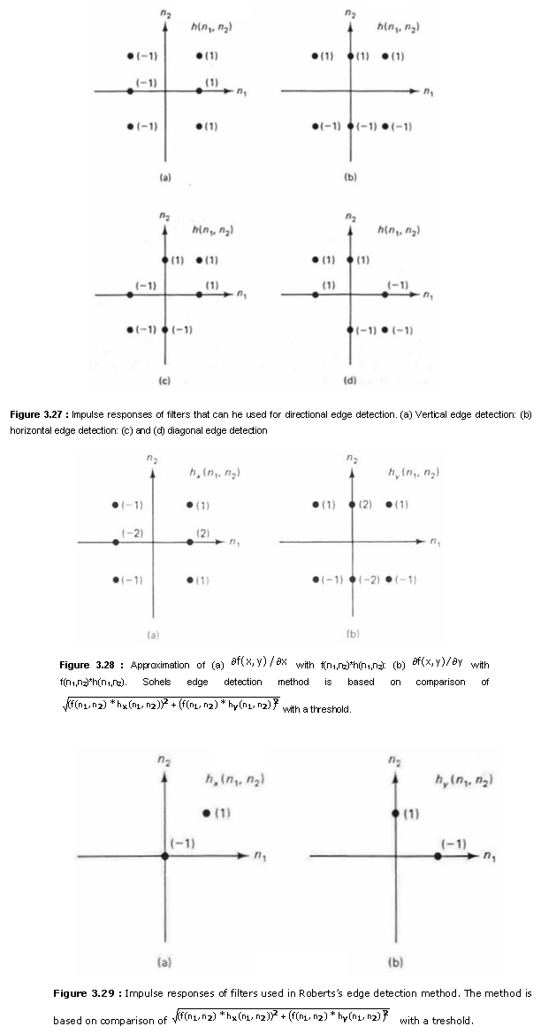
The differencing operation in (3.7) and (3.8) can be viewed as the convolution
of f(n1,n2) with the impulse response of a filter h(n1,n2).
Examples of impulse responses that can be used in developing directional edge
detectors are shown in Figure 3.27. The filters h(n1,n2)
in Figures 3.27(a) and (b) detect edges in the vertical and horizontal
directions and can be viewed as approximating ![]() and
and ![]() respectively. The filters h(n1,n2)
in Figures 3.27(c) and (d) detect edges along the two diagonal directions. The
gradient
respectively. The filters h(n1,n2)
in Figures 3.27(c) and (d) detect edges along the two diagonal directions. The
gradient ![]() in
(3.6) can also be expressed in terms of the first-order partial derivatives in
a rotated coordinate system. When the rotation is 45 degrees, the directions of
partial derivatives are along the two diagonal directions.
in
(3.6) can also be expressed in terms of the first-order partial derivatives in
a rotated coordinate system. When the rotation is 45 degrees, the directions of
partial derivatives are along the two diagonal directions.
Nondirectional edge detectors can be developed by discrete approximation of ![]() in the system in
Figure 3.26. From (3.6).
in the system in
Figure 3.26. From (3.6).
![]() (3.9)
(3.9)
From (3.9), nondirectional edge detectors can be developed by nonlinear combination of the terms used in the development of directional edge detectors. An example of discrete approximation of (3.9) that can be used for nondirectional edge detectors is given by
![]() (3.10)
(3.10)
where
![]()
![]()
and
![]() and
and ![]() are shown in Figure
3.28. The method is based on (3.10) with
are shown in Figure
3.28. The method is based on (3.10) with ![]() and
and ![]() shown in Figure 3.28. Another example is
the method based on (3.10) with
shown in Figure 3.28. Another example is
the method based on (3.10) with ![]() and
and ![]() shown in Figure 3.29. Depending on
exactly how
shown in Figure 3.29. Depending on
exactly how ![]() is
approximated in the discrete domain, many other variations can be developed.
is
approximated in the discrete domain, many other variations can be developed.
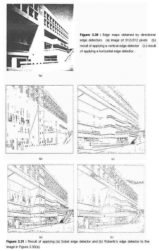
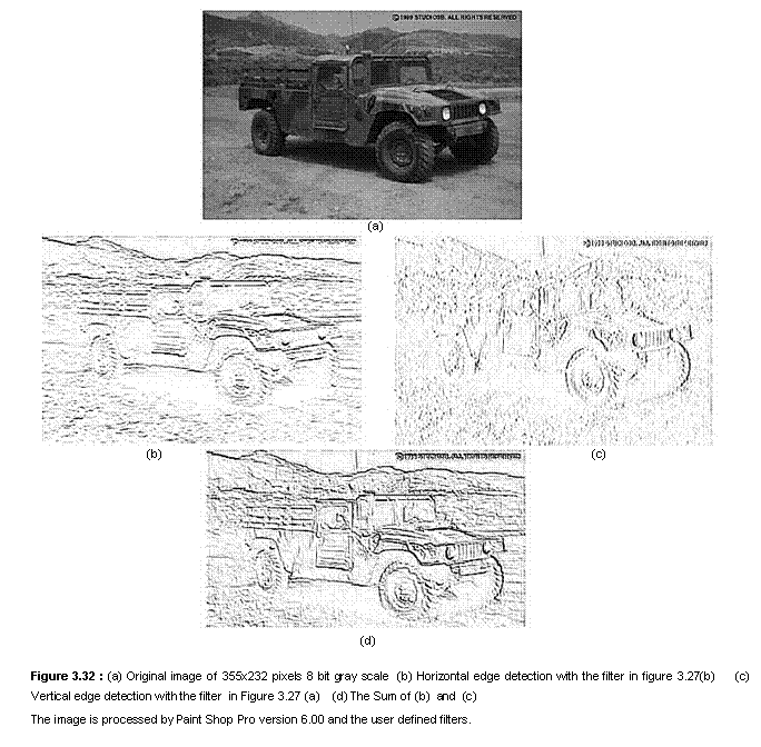
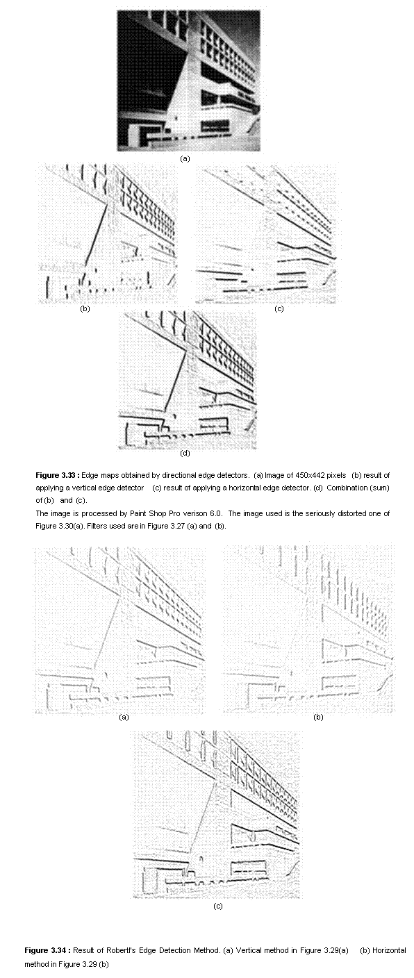
Figure 3.30 shows the result of edge detection using a directional edge detector. Figure 3.30(a) shows an image of 512 x 512 pixels. Figure 3.30(b) and (c) show the results of a vertical edge detector and a horizontal edge detector, respectively, applied to the image in Figure 3.30(a). The vertical and horizontal edge detectors are based on h(n1,n2) in Figures 3.27(a) and (b). Figures 3.3 1(a) and (b) show the results of applying the Sobel edge detector and Roberts’s edge detector to the image in Figure 3.30(a). Both belong to the class of nondirectional edge detectors, and the specific method of determining the threshold value and checking the local maximum property of an edge used is the same as that used in Figure 3.30.
There are many variations of the edge detection methods discussed in this
section. For example, we could use a different nonlinear combination of ![]() and
and ![]() instead of
instead of
![]()
in the system in Figure 3.26. Many different methods can aiso be developed for edge thinning.
The edge detection methods discussed in this section can be improved in various ways. Methods based on computing some form of gradient or differencing are typically sensitive to noise. A certain number of isolated edge points which appear randomly distributed throughout the edge maps in Figure 3.31 are most likely the result of some background noise or very fine image details. Some noise smoothing using the methods discussed in Section 3.2 or more sophisticated noise reduction methods that we will discuss in Chapter 4 may be desirable prior to applying an edge detection algorithm. Isolated random edge points may also be removed by some simple processing of the edge maps. Gradient-based edge detection methods also cause some discontinuities in the detected edge contours, as can be seen from the edge maps in Figure 3.31. Methods that impose continuity constraints in the detected edge contours can also be developed.
