3.2.2. Median Filtering
Median filtering is a nonlinear process useful in reducing impulsive, or salt-and-pepper noise. It is also useful in preserving edges in an image while reducing random noise. Impulsive or salt-and-pepper noise can occur due to a random bit error in a communication channel. In a median filter, a window slides along the image, and the median intensity value of the pixels within the window becomes the output intensity of the pixel being processed. For example, suppose the pixel values within a window are 5, 6, 55, 10, and 15, and the pixel being processed has a value of 55. The output of the median filter at the current pixel location is 10, which is the median of the five values.
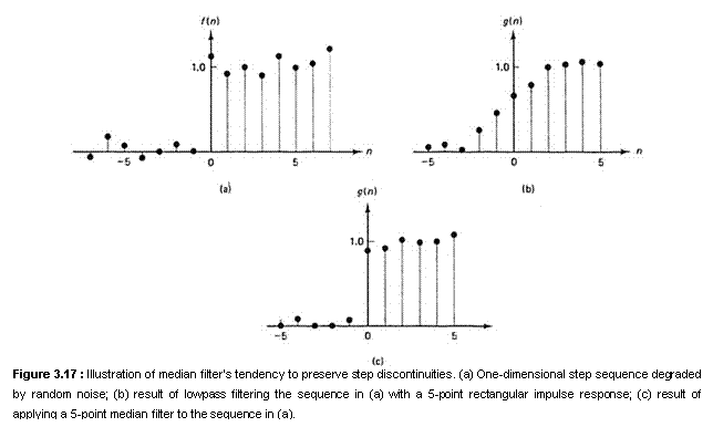
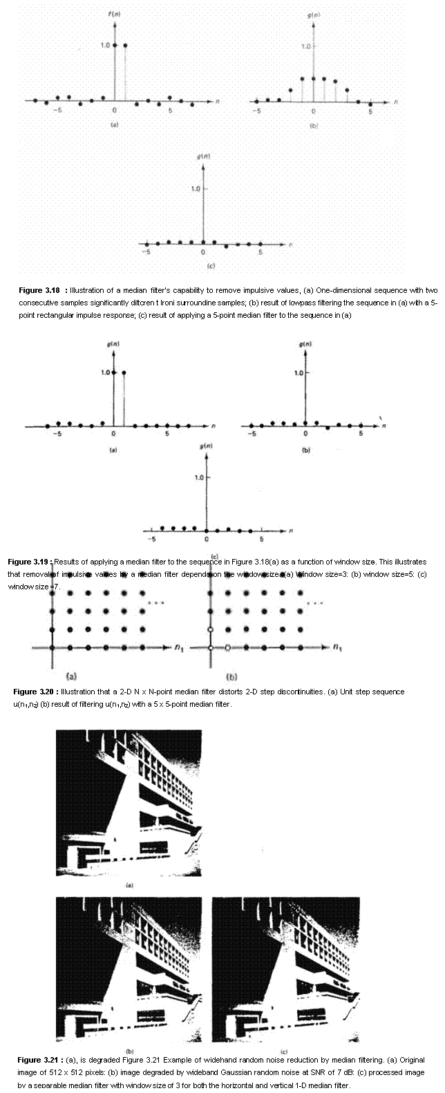
Like lowpass filtering, median filtering smoothes the image and is thus useful in reducing noise. Unlike lowpass filtering, median filtering can preserve discontinuities in a step function and can smooth a few pixels whose values differ significantly from their surroundings without affecting the other pixels. Figure 3.17(a) shows a 1-D step sequence degraded by a small amount of random noise. Figure 3.17(b) shows the result after filtering with a lowpass filter whose impulse response is a 5-point rectangular window. Figure 3.17(c) shows the result after filtering with a 5-point median filter. It is clear from the figure that the step discontinuity is better preserved by the median filter. Figure 3.18(a) shows a 1-D sequence with two values that are significantly different from the surrounding points. Figures 3.18(b) and (c) show the result of a lowpass filter and a median filter, respectively. The filters used in Figure 3.18 are the same as those used in Figure 3.17. If the two impulsive values are due to noise, the result of using a median filter will be to reduce the noise. If the two values are part of the signal, however, using the median filter will distort the signal.
An important parameter in using a median filter is the size of the window. Figure 3.19 illustrates the result of median filtering the signal in Figure 3.18(a) as a function of the window size. If the window size is less than 5, the two pixels with impulsive values will not be significantly affected. For a larger window, they will be. Thus, the choice of the window size depends on the context. Because it is difficult to choose the optimum window size in advance, it may be useful to try several median filters of diflerent window sizes and choose the best of the resulting images.
Median filters are a subset of the class of rank filters where the output image intensity at spatial location x=(x,y)T is chosen on the basis of the relative rank or intensity of pixels in the neighborhood of x. Given a set of N pixel intensities obtained over a local image region, S, denoted simply as fi , i = 1,2, . . . N, an ordering of these values in increasing value, i.e.,
R(x) ={f1,f2,.. .fN} where fi £ fi+1
may be used to derive the rank filter operation. The output image intensity, g(x), is
g(x) = Rankj R(x)
where Rankj is the intensity of the output intensity at position, or rank, j in R(x). For example, choosing j=1 yields the min filter, where the first element of R(x) is chosen; that is,
g(x) = min R(x)
=min {f(x)| x E S}
where S is the chosen neighborhood of x. Alternately, the max filter is derived from choosing j = N and yields
g(x) = max R(x)
=max {f(x)| x E S}
The most popular rank filter is derived for the case of N odd, and is based on choosing the filter output to be fm where m is the median intensity; that is, for N intensity samples the position
m = (N+1)/2
is the median. Thus, fm is the pixel intensity in the ordered sample set that is greater than (N-1)/2 of the samples. We denote the median operator on a sequence of samples as
med (R(x)) = Rank![]() (R(x))
(R(x))
Suppose we obtain N = 5 image intensity samples in a neighborhood of pixel location (x,y) that yield R(x)={100,110,120,130,240}. Clearly the pixel intensity value of 240 is either a noise spike or an image feature. In this case, the output of the rank filter yields g(x) = 120.
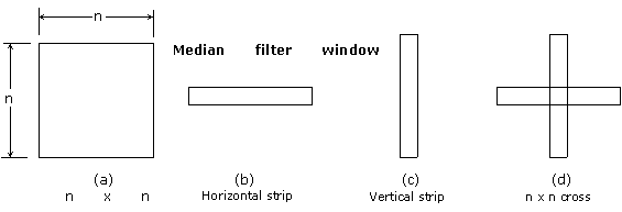
The neighborhood, or window shape, chosen for the median filter greatly affects its filtering effects. The median filter may take an assortment of shapes. Examples are shown in figure. To avoid the computational expense of sorrting large arrays of numbers,median filters often are implemented with a small size window. The image may be repeatedly filtered with multiple passes of this window.
The median operator is a nonlinear filter, because given two image functions yielding sample sequences R1(x) and R2(x),
med (R1(x)+ R2(x)) ¹ med (R1(x))+med (R2(x))
Repeated application of a 1-D median filter to a 1-D sequence eventually leads to a signal called a root signal, which is invariant under further applications of the 1-D median filter. Otherwise a median filter is said to be shift-invariant

In the above, is discussed 1-D median filtering. The task involved in performing a median filtering operation extends straightforwardly from the 1-D case to the 2-D case. However. not all properties of a 1-D median filter apply to a 2-D median filter. For example, median filtering a 1-D unit step sequence u(n) preserves the step discontinuity and does not affect the signal u(n) at all. Suppose we filter a 2-D step sequence u(n1,n2) with a 2-D N x N-point median filter. Figure 3.20(a) shows u(n1,n2) and Figure 3.20(b) shows the result of filtering u(n1,n2) with a 2-D 5 x 5-point median filter. From Figure 3.20(b), the intensity discontinuities which can be viewed as 1-D steps (for large n1 at n2=0 and large n2 at n1=0) are not affected. However, the discontinuities which are truly 2-D steps (n1 = n2 = 0) are seriously distorted. One method that tends to preserve 2-D step discontinuities well is to filter a 2-D signal along the horizontal direction with a 1-D median filter and then filter the result along the vertical direction with another 1-D median filter. This method is called separable median filtering, and is often used in 2-D median filtering applications. When a separable median filter is applied to u(n1,n2), the signal u(n1,n2) is not affected.
A median filter is a nonlinear system, and therefore many theoretical results on linear systems are not applicable. For example, the result of separable median filtering depends on the order in which the 1-D horizontal and vertical median filters are applied. Despite this difficulty, some theoretical results have been developed on median filtering. One result states that repeated application of a 1-D median filter to a 1-D sequence eventually leads to a signal called a root signal, which is invariant under further applications of the 1-D median filter.
Two examples are given to illustrate the performance of a median filter. In the first, the original image of 512 x 512 pixels shown in Figıre 3.21(a), is degraded by wideband Gaussian random noise at an SNR of 7 dB. The degraded image is shown in Figure 3.21(b). Figure 3.21(c) shows the image processed by a separable median filter with a window size of 3 for both the horizontal and vertical 1 -D median filters. Although the very sharp edges are not blurred, median filtering blurs the image significantly. In the second example, the original image from Figure 3.21(a) is degraded by salt-and-pepper noise. The degraded image is shown in Figure 3.22(a) and the image processed by the same separable median filter used in Figure 3.21 is shown in Figure 3.22(b). This example shows that median filtering is quite effective in removing salt-and-pepper noise.


