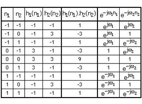
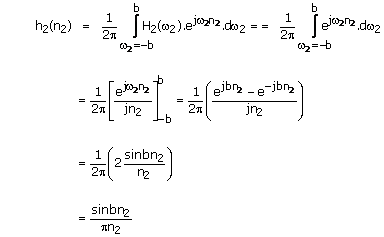
1.3.2 Examples
Example 1
We wish to
determine ![]() for
the sequence h(n1,n2) shown in Figure 1.22(a).
From (1.35).
for
the sequence h(n1,n2) shown in Figure 1.22(a).
From (1.35).


![]()
![]()
![]()
![]()
![]()
![]()
![]()
We knowthat ![]()
And therefore ![]() and
and
![]() can be
written
can be
written
![]()
![]()
![]()

The function ![]() for this example is real
and its magnitude is sketched in Figure 1.22(b). If
for this example is real
and its magnitude is sketched in Figure 1.22(b). If ![]() in Figure
1.22(b) is the frequency response of an LSI system the system corresponds to a
lowpass filter. The function
in Figure
1.22(b) is the frequency response of an LSI system the system corresponds to a
lowpass filter. The function ![]() shows smaller values in
frequency regions away from the origin. A lowpass filter applied to an image
blurs the image. The function
shows smaller values in
frequency regions away from the origin. A lowpass filter applied to an image
blurs the image. The function ![]() is 1 at
is 1 at ![]() and therefore the
average intensity of an image is not affected by the filter. A bright image
will remain bright and a dark image will remain dark after processing with the
filter. Figure 1.23(a) shows an image of
and therefore the
average intensity of an image is not affected by the filter. A bright image
will remain bright and a dark image will remain dark after processing with the
filter. Figure 1.23(a) shows an image of ![]() pixels. Figure 1.23(b) shows the
image obtained by processing the image in Figure 1.23(a) with a lowpass filter
whose impulse response is given by h(n1,n2) in this
example.
pixels. Figure 1.23(b) shows the
image obtained by processing the image in Figure 1.23(a) with a lowpass filter
whose impulse response is given by h(n1,n2) in this
example.
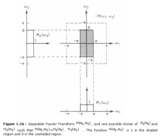
Example 2
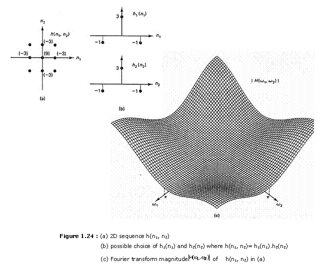
We wish to determine ![]() for the sequence h(n1,n2)
shown in Figure 1.24(a). We can use (1.35) to determine
for the sequence h(n1,n2)
shown in Figure 1.24(a). We can use (1.35) to determine ![]() , as in Example 1.
Alternatively, we can use Property 4 in Table 1.1. The sequence h(n1,n2)
can be expressed as h1(n1)h2(n2)
where one possible choice of h1(n1) and h2(n2)
is shown in Figure 1.24(b). Computing the 1-D Fourier transforms
, as in Example 1.
Alternatively, we can use Property 4 in Table 1.1. The sequence h(n1,n2)
can be expressed as h1(n1)h2(n2)
where one possible choice of h1(n1) and h2(n2)
is shown in Figure 1.24(b). Computing the 1-D Fourier transforms ![]() and
and ![]() and using Property 4 in Table 1.1. we have
and using Property 4 in Table 1.1. we have

![]() ,
,
![]()
Þ 
![]()
The function ![]() is again real, and its
magnitude is sketched in Figure 1.24(c). A system whose frequency response is
given by the
is again real, and its
magnitude is sketched in Figure 1.24(c). A system whose frequency response is
given by the ![]() above is a highpass filter. The
function
above is a highpass filter. The
function ![]() has
smaller values in frequency regions near the origin. A highpass filter applied
to an image tends to accentuate image details or local contrast. and the
processed image appears sharper. Figure 1.25(a) shows an original image of
has
smaller values in frequency regions near the origin. A highpass filter applied
to an image tends to accentuate image details or local contrast. and the
processed image appears sharper. Figure 1.25(a) shows an original image of ![]() pixels and
Figure 1.25(b) shows the highpass filtered image using h(n1,n2)
in this example. When an image is processed. for instance by highpass
filtering, the pixel intensities may no longer he integers between 0 and 255.
They may be negative, noninteger, or above 255. In such instances, we typically
add a bias and then scale and quantize the processed image so that all the
pixel intensities are integers between 0 and 255. It is common practice to
choose the bias and scaling factors such that the minimum intensity is mapped
to 0 and the maximum intensity is mapped to 255.
pixels and
Figure 1.25(b) shows the highpass filtered image using h(n1,n2)
in this example. When an image is processed. for instance by highpass
filtering, the pixel intensities may no longer he integers between 0 and 255.
They may be negative, noninteger, or above 255. In such instances, we typically
add a bias and then scale and quantize the processed image so that all the
pixel intensities are integers between 0 and 255. It is common practice to
choose the bias and scaling factors such that the minimum intensity is mapped
to 0 and the maximum intensity is mapped to 255.
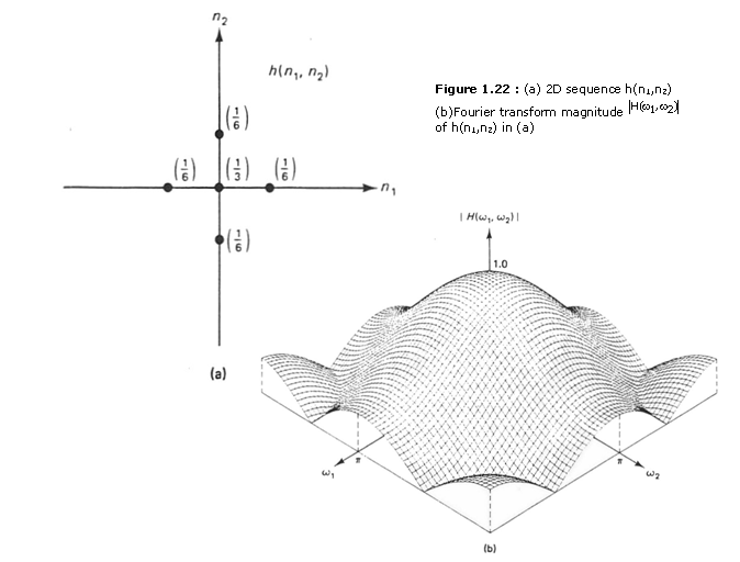
Example 3
We wish to determine h(n1,n2) for
the Fourier transform ![]() shown in Figure 1.23. The
function
shown in Figure 1.23. The
function ![]() is
given by
is
given by
![]()
Since ![]() is always periodic with a period
of 2∏ along each of the two variables
is always periodic with a period
of 2∏ along each of the two variables ![]() and
and ![]() ,
, ![]() is shown only for
is shown only for ![]() £ p and
£ p and ![]() £ p.
The function
£ p.
The function ![]() can be expressed as H(o1)
can be expressed as H(o1)
![]() .
.![]() , where one
possible choice of
, where one
possible choice of ![]() and
and ![]() is also shown in Figure 1.26.
When
is also shown in Figure 1.26.
When
![]() above
is the frequency response of a 2-D LSI system. the system is called a separable
ideal lowpass filter. Computing the 1-D inverse Fourier transforms of
above
is the frequency response of a 2-D LSI system. the system is called a separable
ideal lowpass filter. Computing the 1-D inverse Fourier transforms of ![]() and
and ![]() and using
Property 4 in Table 1.1,we obtain;
and using
Property 4 in Table 1.1,we obtain;
We know by definition that
![]()
And also
![]() =
=![]() .
.![]() &
h(n1, n2) = h1(n1)h2(n2)
&
h(n1, n2) = h1(n1)h2(n2)


And therefore

h(n1,
n2) = h1(n1)h2(n2)=![]()
Example 4
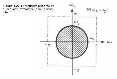
We wish to determine h(n1, n2) for the Fourier
transform ![]() shown
in Figure 1.27. The function
shown
in Figure 1.27. The function ![]() is given by
is given by

When ![]() above is the frequency response
of a 2-D LSI system, the system is called a circularly symmetric ideal
lowpass filter, or an ideal lowpass filter for short. The
inverse Fourier transform of
above is the frequency response
of a 2-D LSI system, the system is called a circularly symmetric ideal
lowpass filter, or an ideal lowpass filter for short. The
inverse Fourier transform of ![]() in this example requires a fair
amount of algebra. The result is
in this example requires a fair
amount of algebra. The result is
![]() h
(1.40)
h
(1.40)
where ![]() represents the Bessel function
of the first kind and the first order and can be expanded in series form as
represents the Bessel function
of the first kind and the first order and can be expanded in series form as
![]() (1.41)
(1.41)
This example shows that 2-D Fourier transform or inverse
Fourier transform operations can become much more algebraically complex than
1-D Fourier transform or inverse Fourier transform operations, despite the fact
that the 2-D Fourier transform pair and many 2-D Fourier transform properties
are straightforward extensions of 1-D results. From (1.40). we observe that the
impulse response of a 2-D circularly symmetric ideal lowpass filter is also
circularly symmetric, that is, it is a function of ![]() . This is a special
case of a more general result. Specifically, if
. This is a special
case of a more general result. Specifically, if ![]() is a function of
is a function of ![]() in the region
in the region
![]() and
is a constant outside the region, then the corresponding h(n1, n2)
is a function of
and
is a constant outside the region, then the corresponding h(n1, n2)
is a function of ![]() . Note, however, that circular
symmetry of h(n1, n2) does not imply circular symmetry of
. Note, however, that circular
symmetry of h(n1, n2) does not imply circular symmetry of
![]() .
The function
.
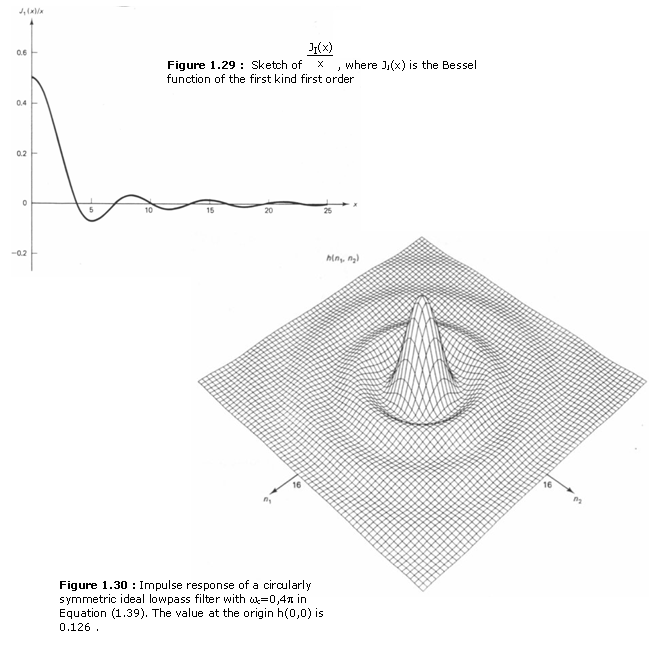
The function![]() is sketched in Figure 1.28. The sequence h(n1, n2) in
(1.40) is sketched in Figure 1 .29 for the case
is sketched in Figure 1.28. The sequence h(n1, n2) in
(1.40) is sketched in Figure 1 .29 for the case ![]() = 0.4∏.
= 0.4∏.
The impulse responses h(n1, n2) obtained from the separable and circularly symmetric ideal lowpass filters in Examples 3 and 4 above are not absolutely sum-
mable, and their Fourier transforms do not converge
uniformly to ![]() used to obtain h(n1,
n2). This is evident from the observation that the two
used to obtain h(n1,
n2). This is evident from the observation that the two ![]() contain
discontinuities and are not analytic functions. Nevertheless, we will regard
them as valid Fourier transform pairs, since they play an important role in
digital filtering and the Fourier transforms of the two h(n1, n2)
converge to
contain
discontinuities and are not analytic functions. Nevertheless, we will regard
them as valid Fourier transform pairs, since they play an important role in
digital filtering and the Fourier transforms of the two h(n1, n2)
converge to ![]() in the mean square sense.
in the mean square sense.