1.2.2 Convolution
The convolution operator in (1.18) has a number of properties that are straightforward extensions of 1-D results. Some of the more important are listed below.
Commutativity: The commutativity property states that the output of an LS1 system is not affected when the input and the impulse response interchange roles.
x(n1, n2)*y(n1, n2)=y(n1, n2)*x(n1, n2) (1.19)
Associativity: The associativity property states that a cascade of two LSI systems with impulse responses h1(n1, n2) and h2(n1, n2) has the same input-output relationship as one LSI system with impulse response h1(n1, n2) * h2(n1, n2).
(x(n1, n2) * y(n1, n2)) * z(n1, n2) = x(n1, n2) * (y(n1, n2) * z(n1, n2)) (1.20)
Distributivity: The distributivity property states that a parallel combination of two LS1 systems with impulse responses h1(n1, n2) and h2(n1, n2) has the same input-output relationship as one LSI system with impulse response given by h1(n1, n2) + h2(n1, n2).
x(n1, n2) * (y(n1, n2) + z(n1, n2))
=(x(n1, n2) *y(n1, n2)) + (x(n1, n2) * z(n1, n2)) (1.21)
Convolution with Shifted impulse : In a special case of (1.22), when m1= m2 = 0, we see that the impulse response of an identity system is d(n1, n2).
x(n1, n2)* d(n1 - m1,n2 - m2) = x(n1 - m1,n2 - m2) (1.22)
The convolution of two sequences x(n1, n2) and h(n1, n2) can be obtained by explicitly evaluating (1.18). It is often simpler and more instructive, however, to evaluate (1.18) graphically. Specifically, the convolution sum in (1.18) can be interpreted as multiplying two sequences x(k1, k2) and h(n1 - k1, n, - k2), which are functions of the variables k1 and k2, and summing the product over all integer values of k1 and k2. The output, which is a function of n1 and n2 , is the result of convolving x(n1, n2) and h(n1, n2).

Figure 1.14 : Example of convolving two sequences
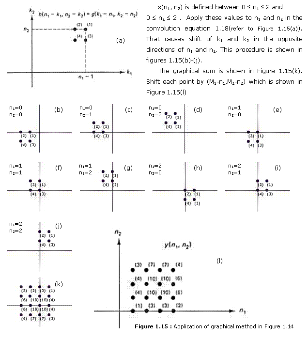
To illustrate, consider the two sequences x(n1, n2) and h(n1, n2) shown in Figures 1.14(a) and (b). From x(n1, n2) and h(n1, n2) , x(k1 , k2) and h(n1 - k1, n2 – k2) as functions of k1 and k2 can be obtained, as shown in Figures 1.14(c)—(f). Note that g(k1 – n1 , k2 – n2) is g(k1, k2) shifted in the positive k1 and k2 directions by n1 and n2 points, respectively. Figures 1.14(d)—(f) show how to obtain h(n1 - k1, n2 - k2) as a function of k1 and k2 from h(n1, n2) in three steps. It is useful to remember how to obtain h(n1 - k1,n2 - k2) directly from h(n1, n2). One simple way is to first change the variables n1 and n2 to k1 and k2 flip the sequence with respect to the origin, and then shift the result in the positive k1 and k2 directions by n1 and n2 points respectively. Once x(k1, k2) and h(n1 - k1, n2 - k2) are obtained they can he multiplied and summed over k1 and k2 to produce the output at each different value of (n1, n2). The result is shown in Figure 1.14(g). The graphical method above is as follows ;
METHOD I : Graphical Method 1
METHOD II : Graphical Method 2
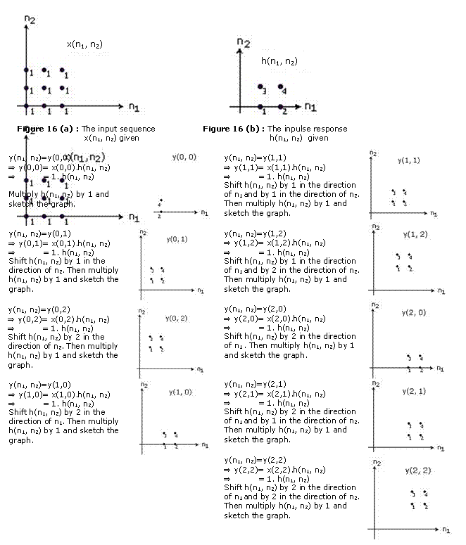
y(n1, n2)=0 outside 0 £ n1 £ 3 , 0 £ n2 £ 3 (Because N=3 , M=2 , N+M-1 = 3+2-1 = 4)
The result is
y(n1, n2)=y(1,0)+ y(1,1)+ y(1,2)+ y(1,3) +y(2,0) +y(2,1)+ y(2,2)+ y(2,3)+ y(2,0)+ y(2,1)+ y(2,2)+ y(3,0)+y(3,1) +y(3,2)+y(3,3) +y(4,0)+y(4,1)+y(4,2)+y(4,3)
This means the sum of 9 graphs sampled above which is as in Figure 1.16(c);

METHOD III :Mathematical Method

Let’s find the value of ![]() at (2,2) ;
at (2,2) ;
y(2,2)![]() 10
10

For each value of
n1 and n2 we calculate ![]() using the same method. The result is the sum of all results.
using the same method. The result is the sum of all results.
Note that because of the commutativity property x(n1, n2)*y(n1, n2)=y(n1, n2)*x(n1, n2) we calculate the same result if we use

instead of

An LSI system is said to be separable, if its impulse response h(n1, n2) is a separable sequence. For a separable system, it is possible to reduce the number of arithmetic operations required to compute the convolution sum. For large-amounts of data. as typically found in images, the computational reduction can be considerable. To illustrate this, consider an input sequence x(n1, n2) of N x N points and an impulse response h(n1, n2) of M x M points:
x(n1, n2) = 0 outside 0 £ n1 £ N – 1 , 0 £ n2 £ N – 1 (1.23)
and
h(n1, n2) = 0 outside 0 £ n1 £ M – 1 , 0 £ n2 £ M - 1
where N » M in typical cases. The regions of (n1, n2) where x(n1, n2) and h(n1, n2) can have nonzero amplitudes are shown in Figures 1.17(a) and (b). The output of the system y(n1, n2), can be expressed as
 (1.24)
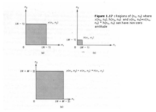
The region of (n1, n2) where y(n1, n2) has nonzero amplitude is shown in Figure 1.17(c).
x(n1, n2)
has N1 x N2 elements, where ![]() and
and ![]() .
.
x(n1, n2) = 0 outside ![]() ,
, ![]() (1.25)
(1.25)
It can also be expressed as ;
x(n1, n2) = 0 outside ![]() ,
, ![]() (1.26)
(1.26)
In the same manner
we can say that h(n1, n2) has M1 x M2
elements ![]() and
and
![]() .
.
h(n1, n2) = 0 outside ![]() ,
, ![]() (1.27)
(1.27)
It can also be expressed as ;
h(n1, n2) = 0 outside ![]() ,
, ![]() (1.28)
(1.28)
The notation ![]() and
and ![]() represents minimum
and maximum values of n1 given.
represents minimum
and maximum values of n1 given.
In this case the graphical limits of y(n1, n2) is defined as ;
having ![]() x
x![]() elements and
elements and
y(n1, n2)=0
outside ![]() ,
,
![]()
If (1.24) is used directly to compute y(n1, n2), approximately (N + M-1)2M2 arithmetic operations (one arithmetic operation = one multiplication and one addition) are required since the number of nonzero output points is (N + M-1)2 and computing each output point requires approximately M2 arithmetic operations. If h(n1, n2) is a separable sequence, it can be expressed as
h(n1, n2) = h1(n1) h2(n2)
h1(n1) = 0 outside 0 £ n1 £ M – 1 , (1.29)
h2(n2) = 0 outside 0 £ n2 £ M – 1 ,
From (1.24) and (1.29) ,
 (1.30)
For a fixed  in (1.26) is a 1-D
convolution of x(k1,n2) and h2(n2).
For example, using the notation
 (1.31)
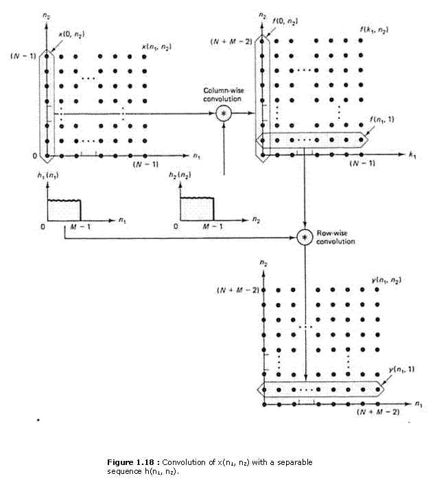
f(0, n2) is the result of 1-D convolution of x(0, n2) with h2(n2). as shown in Figure 1.15. Since there are N different values of k1 for which x(k1, k2) is nonzero, computing f(k1, k2) requires N 1-D convolutions and therefore requires approximately NM(N + M - 1) arithmetic operations. Once f(k1, n2) is computed, y(n1, n2) can be computed from (1.30) and (1.31) by
 (1.32)
From (1.32), for a fixed n2 , y(n1, n2) is a 1-D convolution of h1(n1) and f(n1, n2). For example. y(n1, 1) is the result of a 1-D convolution of f(n1, 1) and h1(n1). as shown in Figure 1.18. where f(n1, n2) is obtained from f(k1, n2) by a simple change of variables. Since there are N + M - 1 different values of n2 ,computing y(n1, n2) from f(k1, n2) requires N + M - 1 1-D convolutions thus approximately M(N + M - 1)2 arithmetic operations. Computing y(n1, n2) from (1.27) and (1.28), exploiting the separability of h(n1, n2), requires approximately NM(N + M — 1) + M(N + M - 1)2 arithmetic operations. This can be a considerable computational saving over (N + M — 1)2 M2. If we assume N» M, exploiting the separability of h(n1, n2) reduces the number of arithmetic operations by approximately a factor of M/2.
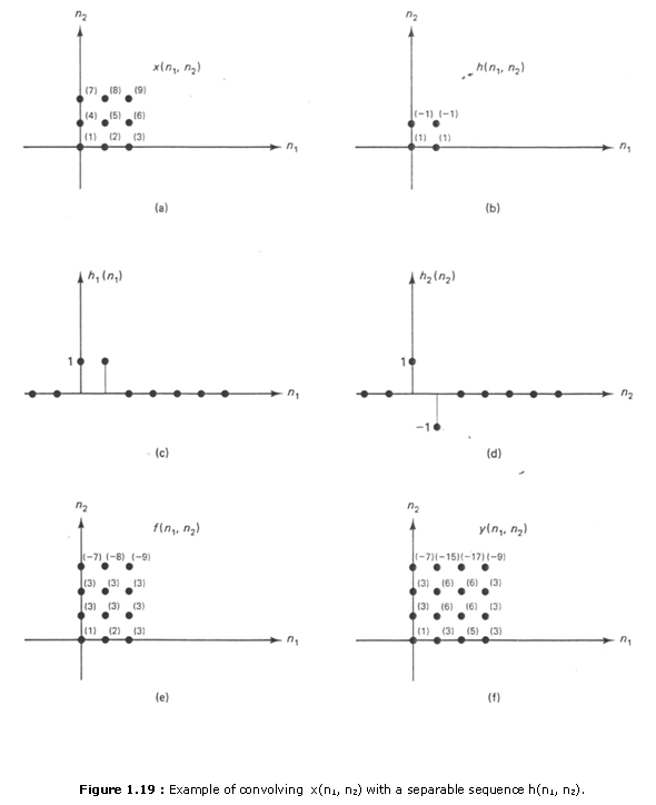
As an example, consider x(n1,n2) and h(n1,n2), shown in Figures 1.19(a) and (b). The sequence h(n1,n2) can he expressed as h1(n1)h2(n2). where h1(n1) and h2(n2) are shown in Figures 1.19(c) and (d), respectively. The sequences f(n1,n2) and y(n1,n2) are shown in Figures 1.19(e) and (f).
In the above discussion, we performed a 1-D convolution first for each column of x(n1,n2) with h2(n2) and then a 1-D convolution for each row of f(n1,n2) with h1(n1). By changing the order of the two summations in (1.30) and following the same procedure. it is simple to show that y(n1,n2) can be computed by performing a 1-D convolution first for each row of x(n1,n2) with h1(n1) and then a 1-D convolution for each column of the result with h2(n2). in the above discussion, we have assumed that x(n1,n2) and h(n1,n2) are N1 x N2-point and M1 X M2-point sequences respectively with N1 = N2 and M1 = M2 We note that the results discussed above can be generalized straightforwardly to the case when N1 ¹ N2 and M1 ¹ M2.
