2 DSP Review
2.1 Basics
Digital Signal Processing (DSP) is used in a wide variety of applications, and it is hard to find a good definition that is general. We can start by dictionary definitions of the words. Digital is operating by the use of discrete signals to represent data in the form of numbers. Signal is a variable parameter by which information is conveyed through an electronic circuit. Processing is to perform operations on data according to programmed instructions. This leads us to a simple definition: Digital Signal processing is changing or analyzing information which is measured as discrete sequences of numbers. Note two unique features of Digital Signal processing as opposed to plain old ordinary digital processing: signals come from the real world - this intimate connection with the real world leads to many unique needs such as the need to react in real time and a need to measure signals and convert them to digital numbers, and signals are discrete - which means the information in between discrete samples is lost.
The advantages of DSP are common to many digital systems and include versatility, repeatability, and simplicity. Versatility: digital systems can be reprogrammed for other applications (at least where programmable DSP chips are used) and digital systems can be ported to different hardware (for example a different DSP chip or board level product). Repeatability: digital systems can be easily duplicated, digital systems do not depend on strict component tolerances, and digital system responses do not drift with temperature. Simplicity: some things can be done more easily digitally than with analogue systems.
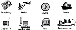
Figure 2‑1: Applications of Digital Signal Processing.
DSP is used in a very wide variety of applications (Figure 2‑1) but most share some common features: they use a lot of maths (multiplying and adding signals), they deal with signals that come from the real world, and they require a response in a certain time. Where general purpose DSP processors are concerned, most applications deal with signal frequencies that are in the audio range.
2.2 Converting Analogue Signals
Most DSP applications deal with analogue signals where the analogue signal has to be converted to digital form as shown in Figure 2‑2. The analogue signal - a continuous variable defined with infinite precision - is converted to a discrete sequence of measured values which are represented digitally. Information is lost in converting from analogue to digital, due to: inaccuracies in the measurement, uncertainty in timing, and the limits on the duration of the measurement. These effects are called quantization errors.
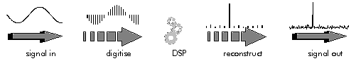
Figure 2‑2: The analog to digital process of DSP.
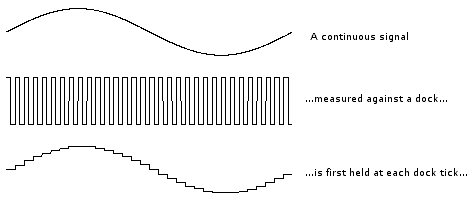
Figure 2‑3: Digitization of an analog signal.
The continuous analogue signal has to be held before it can be sampled. Otherwise, the signal would be changing during the measurement. Only after it has been held can the signal be measured, and the measurement converted to a digital value (Figure 2‑3).
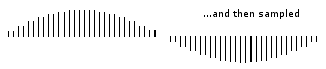
Figure 2‑4: Sampled signal.
The sampling results in a discrete set of digital numbers that represent measurements of the signal - usually taken at equal intervals of time (Figure 2‑4). Note that the sampling takes place after the hold. This means that we can sometimes use a slower Analogue to Digital Converter (ADC) than might seem required at first sight. The hold circuit must act fast enough that the signal is not changing during the time the circuit is acquiring the signal value, but the ADC has all the time that the signal is held to make its conversion. We don't know what we don't measure. In the process of measuring the signal, some information is lost (Figure 2‑5). Sometimes we may have some a priori knowledge of the signal, or be able to make some assumptions that will let us reconstruct the lost information.
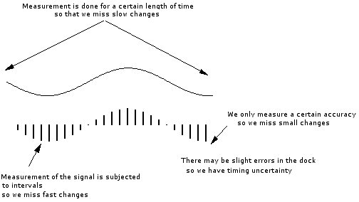
Figure 2‑5: The loss of information during sampling.
2.3 Aliasing
We only sample the signal at intervals that we don't know what happened between the samples. A crude example is to consider a 'glitch' that happened to fall between adjacent samples. Since we don't measure it, we have no way of knowing the glitch was there at all.
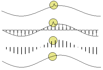
Figure 2‑6: The aliasing artifact. Loss of information.
In a less obvious case, we might have signal components that are varying rapidly in between samples. Again, we could not track these rapid inter-sample variations (Figure 2‑6). Therefore, we must sample fast enough to see the most rapid changes in the signal. Sometimes we may have some a priori knowledge of the signal, or be able to make some assumptions about how the signal behaves in between samples. If we do not sample fast enough, we cannot track completely the most rapid changes in the signal.
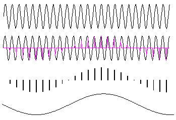
Figure 2‑7: Sampling at slow rates.
Some higher frequencies can be incorrectly interpreted as lower ones. In Figure 2‑7, the high frequency signal is sampled just under twice every cycle. The result is that each sample is taken at a slightly later part of the cycle. If we draw a smooth connecting line between the samples, the resulting curve looks like a lower frequency. This is called 'aliasing' because one frequency looks like another.
Note that the problem of aliasing is that we cannot tell which frequency we have - a high frequency looks like a low one so we cannot tell the two apart. But sometimes we may have some a priori knowledge of the signal, or be able to make some assumptions about how the signal behaves in between samples, that will allow us to tell unambiguously what we have.
Nyquist showed that to distinguish unambiguously between all signal frequency components we must sample faster than twice the frequency of the highest frequency component.
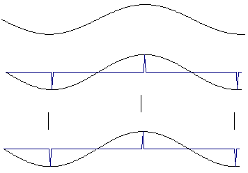
Figure 2‑8: Sampling high frequency signal. A continuous signal sampled twice per cycle has enough information to be reconstructed.
In Figure 2‑8, the high frequency signal is sampled twice every cycle. If we draw a smooth connecting line between the samples, the resulting curve looks like the original signal. But if the samples happened to fall at the zero crossings, we would see no signal at all - this is why the sampling theorem demands we sample faster than twice the highest signal frequency. This avoids aliasing. The highest signal frequency allowed for a given sample rate is called the Nyquist frequency. Actually, Nyquist says that we have to sample faster than the signal bandwidth, not the highest frequency. But this leads us into multirate signal processing which is a more advanced subject.
2.4 Antialiasing
Nyquist showed that to distinguish unambiguously between all signal frequency components we must sample at least twice the frequency of the highest frequency component. To avoid aliasing, we simply filter out all the high frequency components before sampling (Figure 2‑9).
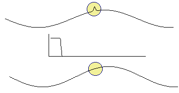
Figure 2‑9: The effect of antialiasing filter. High frequency components are removed through a low pass filter.
Note that antialias filters must be analogue - it is too late once you have done the sampling. This simple brute force method avoids the problem of aliasing. But it does remove information - if the signal had high frequency components, we cannot now know anything about them.
Although Nyquist showed that provide we sample at least twice the highest signal frequency we have all the information needed to reconstruct the signal, the sampling theorem does not say the samples will look like the signal.
Figure 2‑10: A high frequency signal sampled fast enough may still look wrong but can be reconstructed.
Figure 2‑10 shows a high frequency sine wave that is nevertheless sampled fast enough according to Nyquist's sampling theorem - just more than twice per cycle. When straight lines are drawn between the samples, the signal's frequency is indeed evident - but it looks as though the signal is amplitude modulated. This effect arises because each sample is taken at a slightly earlier part of the cycle. Unlike aliasing, the effect does not change the apparent signal frequency. The answer lies in the fact that the sampling theorem says there is enough information to reconstruct the signal - and the correct reconstruction is not just to draw straight lines between samples.
The signal is properly reconstructed from the samples by low pass filtering: the low pass filter should be the same as the original antialias filter. The reconstruction filter interpolates between the samples to make a smoothly varying analogue signal. In Figure 2‑11, the reconstruction filter interpolates between samples in a 'peaky' way that seems at first sight to be strange. The explanation lies in the shape of the reconstruction filter's impulse response.
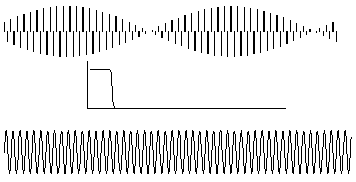
Figure 2‑11: A sampled signal must be low-pass filtered to reconstruct the original.
The impulse response of the reconstruction filter has a classic 'sin(x)/x shape. The stimulus fed to this filter is the series of discrete impulses which are the samples. Every time an impulse hits the filter, we get 'ringing' - and it is the superposition of all these peaky rings that reconstructs the proper signal. If the signal contains frequency components that are close to the Nyquist, then the reconstruction filter has to be very sharp indeed. This means it will have a very long impulse response - and so the long 'memory' needed to fill in the signal even in region of the low amplitude samples.
2.5 Frequency resolution
Sampling of the signal is done only for a certain time. We cannot see slow changes in the signal if we don't wait long enough. In fact we must sample for long enough to detect not only low frequencies in the signal, but also small differences between frequencies. The length of time for which we are prepared to sample the signal determines our ability to resolve adjacent frequencies - the frequency resolution.
We must sample for at least one complete cycle of the lowest frequency we want to resolve. We can see that we face a forced compromise. We must sample fast to avoid and for a long time to achieve a good frequency resolution. But sampling fast for a long time means we will have a lot of samples - and lots of samples means lots of computation, for which we generally don't have time. So we will have to compromise between resolving frequency components of the signal, and being able to see high frequencies.
2.6 Quantization
When the signal is converted to digital form, the precision is limited by the number of bits available. Figure 2‑12 shows an analogue signal which is then converted to a digital representation - in this case, with 8 bit precision. The smoothly varying analogue signal can only be represented as a 'stepped' waveform due to the limited precision. Sadly, the errors introduced by digitization are both non linear and signal dependent. Non linear means we cannot calculate their effects using normal math. Signal dependent means the errors are coherent and so cannot be reduced by simple means.
This is a common problem in DSP. The errors due to limited precision (i.e. word length) are non linear (hence incalculable) and signal dependent (hence coherent). Both are bad news, and mean that we cannot really calculate how a DSP algorithm will perform in limited precision - the only reliable way is to implement it, and test it against signals of the type expected. The non linearity can also lead to instability - particularly with IIR filters. The word length of hardware used for DSP processing determines the available precision and dynamic range.
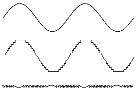
Figure 2‑12: Limited precision leads to errors which are signal dependent.
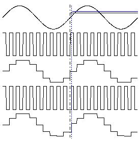
Figure 2‑13: Timing error leads to value error, an accurate dock leads to accurate values. An error in the dock translates the error in the values.
Uncertainty in the clock timing leads to errors in the sampled signal. Figure 2‑13 shows an analogue signal which is held on the rising edge of a clock signal. If the clock edge occurs at a different time than expected, the signal will be held at the wrong value. Sadly, the errors introduced by timing error are both non linear and signal dependent.
A real DSP system suffers from three sources of error due to limited word length in the measurement and processing of the signal: limited precision due to word length when the analogue signal is converted to digital form, errors in arithmetic due to limited precision within the processor itself, and limited precision due to word length when the digital samples are converted back to analogue form.
These errors are often called quantization error. The effects of quantization error are in fact both non linear and signal dependent. Non linear means we cannot calculate their effects using normal math. Signal dependent means that even if we could calculate their effect, we would have to do so separately for every type of signal we expect. A simple way to get an idea of the effects of limited word length is to model each of the sources of quantization error as if it were a source of random noise.
The model of quantization as injections of random noise is helpful in gaining an idea of the effects. But it is not actually accurate, especially for systems with feedback like IIR filters. The effect of quantization error is often similar to an injection of random noise.
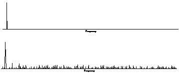
Figure 2‑14: Quantization error. The spectrum of a pure tone is noisy when quantized.
Figure 2‑14 shows the spectrum calculated from a pure tone. The top plot shows the spectrum with high precision (double precision floating point) and the bottom plot shows the spectrum when the sine wave is quantized to 16 bits. The effect looks very like low level random noise. The signal to noise ratio is affected by the number of bits in the data format, and by whether the data is fixed point or floating point.
2.7 Summary
A DSP system has three fundamental sources of limitation:
- loss of information because we only take samples of the signal at intervals
- loss of information because we only sample the signal for a certain length of time
- errors due to limited precision (i.e. word length) in data storage and arithmetic
The effects of these limitations are as follows:
- aliasing is the result of sampling, which means we cannot distinguish between high and low frequencies
- limited frequency resolution is the result of limited duration of sampling, which means we cannot distinguish between adjacent frequencies
- quantization error is the result of limited precision (word length) when converting between analogue and digital forms, when storing data, or when performing arithmetic
Aliasing and frequency resolution are fundamental limitations - they arise from the mathematics and cannot be overcome. They are limitations of any sampled data system, not just digital ones.
Quantization error is an artifact of the imperfect precision, and can be improved upon by using an increased word length. It is a feature peculiar to digital systems. Its effects are non linear and signal dependent, but can sometimes be acceptably modeled as injections of random noise.