3 Framework
3.1 Introduction
This chapter gives the basics of the volume-rendering algorithm which will be the subject of the hardware implementation. It is basically a template-based, discrete ray tracing algorithm. Discrete ray tracing is well known and common in use as it prefers discrete representations of models rather than geometric forms, which therefore provides a substantial improvement in computational speed. “Template” refers to the ray to be traced for every pixel on the image plane into the volume to find the contribution of the data for that pixel. It is an important optimization method for volume rendering. Rays skips empty voxel space, providing a significant speed-up without affecting the image quality, which is also an important optimization of the algorithm and known as space leaping.
3.2 The Pipeline
The rendering pipeline of the visualization algorithm is shown in Figure 3‑1. The organization scheme of the memory module affects the performance of rendering algorithms. The volumetric dataset to be rendered is provided in a standard memory module. It is possible to say that the algorithm suffers from the limited memory performance capabilities of personal computers. To decrease this burden, an 8-bit data structure per voxel is used in the majority of the datasets. Still it is obvious that the speed of a ray-caster depends on the total number of voxels it traverses. Thus, the total rendering time of a volume is a matter of volume resolution, independent of the object complexity within the volume.
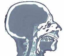
Slice extraction is the cheapest part of the pipeline, as it requires nothing but just accessing the correct addresses of the volume data to generate an image. Slice images can be generated in arbitrary angles with each of the spatial axes. Examples are shown in Figure 3‑2.
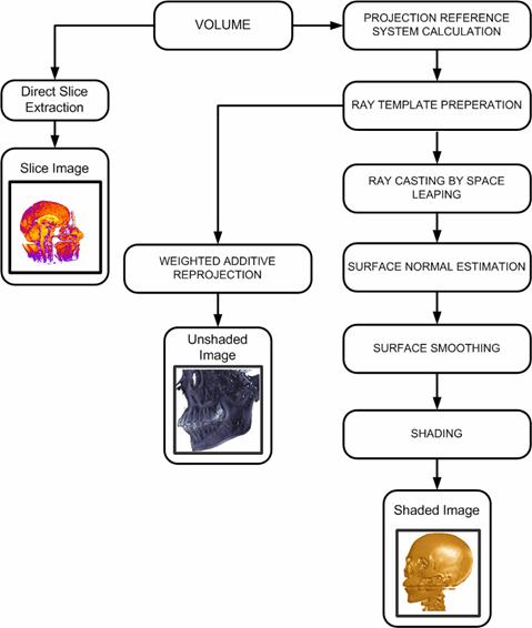
Figure 3‑1: The pipeline of the algorithm
(a) (b)
Figure 3‑2: Slices extracted from the CT dataset. a. Sagittal view, b. axial view
The projection reference system is standard for all graphics applications. The planar geometric projection used by the algorithm is orthogonal projection as it simplifies the algorithm by giving rise to the inter-ray coherency. But spatial address transformation, surface normal estimation, space leaping, and surface smoothing algorithms that are going to be introduced later are applicable for perspective projection as well.
Since parallel projection is used, the direction of projection and the normal to the projection plane are the same in direction. Therefore, all rays have the same form. A discrete line algorithm is activated once per projection, and its elements are recorded in a data structure called ray template, which is essentially a line with 26-connectivity. The usage of the template provides a considerable time/performance benefit to the system. However, this strategy causes the skipping of some voxels for 26-rays, while some others are being visited twice. This phenomenon leads to the employment of a plane other than the view plane, parallel to one of the principle axes, and tracing templates from that plane. It is called base-plane. It was determined which of the volume faces projected to the largest area on the screen-plane that the plane containing this face as the base-plane. The volume is projected onto the base-plane and then perform a 2D image transformation to yield the desired result. The base-plane used in this work is oriented as near as possible to the actual view plane while preserving its parallelism to one of the spatial axes. This leads to the minimization of projection errors originated from the base-plane usage, and therefore eliminates the need for a 2D transformation.
(a) (b)
Figure 3‑3: Images generated by two different tracing schemes. a. First-hit projection method, b. weighted additive reprojection method
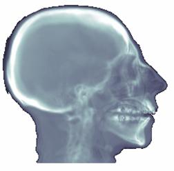
Commonly, the outcome of the viewing process consists of, for each screen pixel, the depth and the value (color) of the first opaque voxel encountered by the ray emitted from that pixel. This scheme is called first-hit projection. However, it is possible to apply different operators while following the ray. The weighted additive reprojection produces an X-ray-like image by averaging the intensities along the ray. Alternatively, one could display the maximum value encountered along the ray passage, like in a method called maximum projection, or the minimum value encountered called minimum intensity projection. Assigning opacities to voxel values will enable a compositing projection to simulate semitransparent volumes. Two samples are shown in Figure 3‑3. The left image is a first-hit projection without shading and the image on the right is produced by the weighted additive reprojection method. The first opaque voxels found during tracing are provided as input for the shading process
The traversal of volume data consists of two phases, the traversal of the empty space, and the traversal of the occupied voxels. It is obvious that the empty space does not have to be sampled – it has only to be crossed as fast as possible. For all the ray traversal schemes that are included into this pipeline, the empty space is leaped forward. There are many methods that apply to space leaping in the literature. Existing methods require a preprocessing stage, and some require specific rendering methods. Here, a method that independent of the rendering algorithm is used.
Most ray tracing schemes require a shading model to be used to enhance the understanding of the data. For each voxel, a normal vector is required for the shading stage. As the data in the volume is represented in discrete space, no geometric information is available explicitly, which yields a lack of information. Therefore, a normal vector to the surface of each voxel has to be estimated. This process is called surface-normal estimation. The usage of gradient vector instead of the surface normal is the trend in volume rendering literature.
(a) (b)
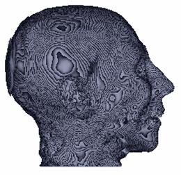
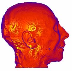
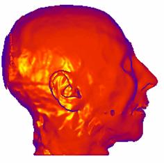
Figure 3‑4: Shaded image of CT dataset. a. Without surface-smoothing, b. with surface smoothing
The method used for the normal estimation, is based on a simple geometric model of the voxel neighborhood. Five polygons are produced from the four neighbors of each voxel and the normal is estimated by averaging these polygon normals. The discrete representation of the data causes an incorrect, patch-like shaded image with the surface normals estimated, as shown in Figure 3‑4.a, and the process of repairing these patches is called surface smoothing. There are several methods in the literature. The method introduced in this work is based on averaging the surface normals exceeding a threshold within a pre-defined kernel. An image with surface smoothing is shown in Figure 3‑4.b. The Phong shading is preferred as the shading model.
3.3 Specification of an Arbitrary 3D View
In general, projections transform points in a coordinate system of dimension n into points in a coordinate system of dimension less than n. In fact, computer graphics has long been used for studying n-dimensional objects by projecting them into 2D for viewing. The projection of a 3D object is defined by straight projection rays, emanating from a center of projection, passing through each point of the object, and intersecting a projection plane to form the projection. The class of projections with which we deal with is known as planar geometric projections. Planar geometric projections can be divided into two basic classes: perspective and parallel. The distinction lies in the relation of the center of projection to the projection plane. If the distance from the one to the other is finite, then the projection is perspective, and if infinite the projection is parallel. When we define a perspective projection, we explicitly specify its center of projection; for a parallel projection, we give its direction of projection. The visual effect of a perspective projection is similar to that of photographic systems and of the human visual system, and is known as perspective foreshortening. The size of the perspective shortening of an object varies inversely with the distance of that object from the center of projection. Thus, although the perspective projection of objects tends to look realistic, it is not particularly useful for recording the exact shape and measurements of the objects; distances cannot be taken from the projection, angles are preserved on only those faces of the object parallel to the projection plane, and parallel lines do not in general project as parallel lines. The parallel projection is a less realistic view because perspective foreshortening is lacking, although there can be different constant foreshortenings along each axis. The projection can be used for exact measurements, and parallel lines do remain parallel. As in the perspective projection, angles are preserved only on faces of the object parallel to the projection plane.
In order to specify an orthographic projection system:
· A reference point on the plane is defined (view reference point VRP )(Figure 3‑5),
· a normal to the plane is defined ( view plane normal VPN ) (Figure 3‑5),
· an up vector is defined (view-up vector VUP) (Figure 3‑6),
· using VRP and VPN, the view plane is calculated,
· the v-axis of the plane is calculated,
· the u-axis of the plane is calculated, (Figure 3‑7) and,
· a window on the plane is defined whose contents are mapped to the viewport for visualization.(Figure 3‑8)
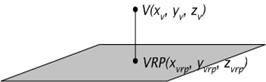
Figure 3‑5: View reference point (VRP) and point V on the view plane
Figure 3‑6: Definition of the view-up vector
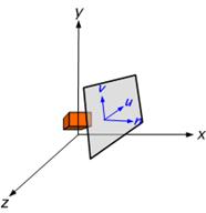
Figure 3‑7: The components of an orthographic projection system
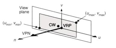
Figure 3‑8: The definition of the window on the view plane
3.4 Ray Template
Voxelization algorithms that convert a 3D continuous line representation into a discrete line representation have two common usages in volume graphics:
1. As the 3D line is a fundamental primitive, it is used as a building block for generating more complex objects. For example, a voxelized cylinder can be generated by sweeping a 3D voxelized circle.
2. It is used for ray traversal in the voxel space. Rendering techniques that cast rays through a volume of voxels are based on algorithms that generate the set of voxels visited by the continuous ray. Discrete ray algorithms have been developed for the traversal of a 3D space partition.
A formal definition of a 3D discrete line is mandatory in numerous applications. The existing methods may be sorted in two categories as:
1. “By projections” method, where two projections of the 3D segment are independently computed on two basic planes, (Figure 3‑9),
2. “By direct calculus” method obtained by an extension of the 2D and 3D algorithms.
A line voxelization algorithm generates a 3D discrete line from a 3D continuous line, which is a set of connected voxels approximating the continuous line.
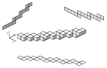
Figure 3‑9: By projections generation method of a 3D discrete line
3.5 Shading
As a result of first-hit projection the data seized by the traced rays are projected onto the view plane. But it is obvious from Figure 3‑4.a that, the image is unpleasant and it cannot support perception. Realistic displays of data can amplify cognition and they can be obtained by applying natural lighting effects to the visible surfaces. An illumination model is used to calculate the intensity of light that should be seen at a given point on the surface of the object. The model developed by Bui-Tuong Phong is preferred as it yields substantial improvements over other models and known as Phong illumination model.
Modeling the colors and lighting effects that is seen on an object is a complex process, involving principles of physics and psychology. Fundamentally, lighting effects are described with a model that considers the interaction of electromagnetic energy with object surfaces. Once light reaches the observer’s eyes, it triggers perception processes that determine what is actually seen in a scene. Phong illumination model involves a number of factors, such as object type, object position relative to light source and other objects, and the light source conditions that are defined for the scene. Objects can be constructed from opaque materials, or they can be more or less transparent. In addition, they can have shiny or dull surfaces, and they can have a variety of surface-texture patterns. Light sources, of varying shapes, colors, and positions, can be used to provide the illumination effects for an image. Given the parameters for the optical properties of surfaces, the relative positions of the surfaces in a scene, the color and positions of the light sources, and the position and orientation of the viewing plane, Phong model calculates the intensity projected from a particular surface point in a specified viewing direction.
Figure 3‑10 and Figure 3‑11 shows the effect of different parameters of shading algorithm, and Figure 3‑12 shows the combined result of shading parameters.
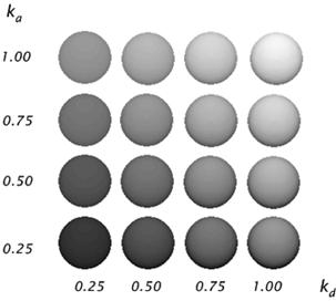
Figure 3‑10: Diffuse reflections from a spherical surface illuminated with ambient light and a single point light source for values of ka and kd in the interval (0, 1).
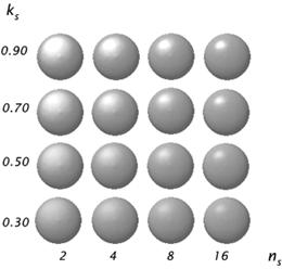
Figure 3‑11: Specular reflections from a spherical surface for varying specular parameter values and a single light source.
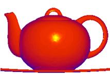
Figure 3‑12: A color model shaded using Phong shading. Diffuse and specular reflections are combined to obtain a complete shading model.
In this chapter, the general structure of the subject of this hardware implementation is presented in a pipelined manner. This pipeline combines several algorithms to extract meaningful information from the given data. The reference of the projection system is almost standard for all graphics applications. Address space transformation is the major subject of this reference system.
The first-hit projection scheme employs ray tracing, which involves an illumination model. A 3D line generator calculates the common form of the rays to be traced. Phong model is used for shading as it provides substantial improvements over the other existing methods. The implementation of a global illumination algorithm invites the normal vectors at each sampling point in the final image. Since there are no such explicit information available with discrete representation scheme of the data, these vectors has to be approximated. This is done with a surface normal estimation algorithm. As a drawback, the final image suffers from some undesired effects, which have to be repaired. The existence of a surface-smoothing algorithm in the pipeline stem from this need. It discards these artifacts and produces pleasing images.
In this chapter, we have also reviewed the methods used in the specification of an arbitrary view, the 3D line generation and the construction of the ray template, and the shading algorithms in detail.